Judgment and Decision Making, Vol. 13, No. 6, November 2018, pp. 587-606
Boundary effects in the Marschak-Machina triangle
Krzysztof Kontek*
|
This paper presents the results of a study that sheds new light on
the shape of indifference curves in the Marschak-Machina triangle. The
most important observation, obtained non-parametrically, concerns jumps
in indifference curves at the triangle legs towards the triangle
origin. These jumps, however, do not appear at the hypotenuse. The
pattern observed suggests discontinuity in lottery valuation when the
range of lottery outcomes changes and is best explained by
decision-making models based on the psychological phenomenon of range
dependence (Parducci, 1965; Cohen, 1992; Kontek & Lewandowski, 2018).
Models founded on other psychological phenomena, e.g., discontinuity in
decision weights (Kahneman & Tversky, 1979), cumulative probability
weighting (Tversky & Kahneman, 1992), attention shifting (Birnbaum,
2008), overweighting of salient payoffs (Bordallo, Gennaioli & Shefrin,
2012), and treating stated probabilities as imperfect information
(Viscusi, 1989), predict indifference curve shapes that differ from the
one obtained in this study.
Keywords: Marschak-Machina triangle, indifference curves, certainty equivalents,
trimmed mean, models of decision-making under risk, ranking of models
1 Introduction
The Marschak-Machina triangle (Marschak, 1950; Machina, 1982) is a
graphical tool for both theoretical and experimental considerations
concerning the modeling of decision-making under risk. The triangle
represents the set of all lotteries involving three fixed outcomes
x1<x2<x3 with respective probabilities of p1, p2, and
p3. Probability p1 is represented on the horizontal axis;
probability p3 is represented on the vertical axis; and
probability p2 is their sum subtracted from 1. Every point in this
triangle represents a particular lottery: a point inside the triangle
represents a three-outcome lottery where p1, p2, and p3
are strictly positive; a point on the boundary of the triangle (but not
at one of the corners) represents a two-outcome lottery, since one
pi is zero; while the corners represent certainties.
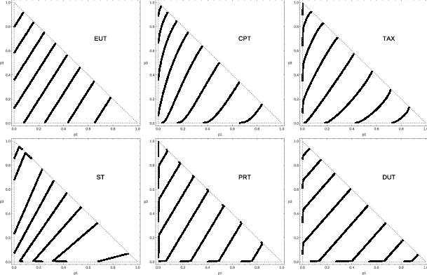
| Figure 1: Indifference curve shapes predicted by: Expected Utility Theory (EUT,
von Neumann and Morgenstern, 1944), Cumulative Prospect Theory (CPT,
Tversky & Kahneman, 1992), the TAX model (TAX, Birnbaum, 2008),
Salience Theory (ST, Bordalo, Gennaioli, and Shefrin, 2012),
Prospective Reference Theory (PRT, Viscusi, 1989), and the Decision
Utility model (DUT, Kontek and Lewandowski, 2018). |
A common and useful way to visualize the predictions of the various
decision-making models is to inspect their indifference curves, as they
connect points representing lotteries of equal utility. If the
decision-maker behaves in accordance with Expected Utility Theory (von
Neumann & Morgenstern, 1944), then his or her preferences can be
represented in the Marschak-Machina triangle by a set of parallel
straight line indifference curves. A number of theories of
decision-making under risk have been developed to explain Expected
Utility violations (more specifically the Allais paradox). These models
predict indifference curves of various shapes: straight lines that
“fan-out” (i.e., that intersect at a point to the south-west of the
triangle origin, Chew & MacCrimmon, 1979; Loomes & Sugden, 1982),
“fan-in” (i.e., that intersect at a point to the north-east of the
hypotenuse, Blavatskyy, 2006), are a mixture of both (Gul, 1991;
Neilson, 1992; Jia et al., 2001; Bordalo, Gennaioli & Schleifer, 2012),
or do not converge to any specific point (Dekel, 1986). The
indifference curves may be concave (Kahneman and Tversky, 1979),
concave or convex (Becker, Sarin, 1987), or concave and convex
(Tversky & Kahneman, 1992; Birnbaum, 2008). They may also be
discontinuous at all boundaries (Kahneman & Tversky, 1979; Viscusi,
1989; Birnbaum, 2008; Bordalo, Gennaioli, Schleifer, 2012), or only at
the triangle legs (Cohen, 1992; Kontek & Lewandowski, 2018). The
Marschak-Machina triangle, with the indifference curves inside it, is
therefore a powerful tool for distinguishing the predictions of
different decision-making models. Example shapes of the indifference
curves predicted by the models discussed in this paper are presented in
Figure 1.
Many investigations have tested hypotheses about the shape of the
indifference map using real data (e.g., Hey & Strazzera, 1989; Camerer,
1989; Loomes, 1991; Harless, 1992; Blavatskyy, 2006; Bardsley et al.,
2010). Harless and Camerer (1994), after analyzing a large number of
experimental data sets, conclude that the EU model should be used when all
the lotteries are located in the interior of the triangle (from which
follows that the indifference curves are parallel straight lines inside the
triangle), but a different model has to be used when some of the lotteries
are located on the boundaries or in the corners of the triangle. The
literature contains evidence of boundary effects (e.g., Conlisk, 1989),
although the shape of the indifference curves in the vicinity of the
triangle boundaries is not clearly stated. For instance, Abdellaoui and
Munier (1998) state only that the hypothesis concerning parallelism of the
indifference curves at the triangle legs is strongly rejected.
This paper presents the results of a study that sheds new light on the
shape of indifference curves in the Marschak-Machina triangle. The study
was performed using a novel method of non-parametrically plotting
indifference curves using certainty equivalents based on the common
cartographic practice of plotting contour maps (Section
??). The approach allows the indifference curves to be
visualized (Section ??) in contrast to most previous
studies, which tested only hypotheses about the shapes of the indifference
curves in the entire triangle or in its regions (Section
??). Importantly, many of the lotteries considered in
the present study were located close to the Marschak-Machina triangle
boundaries (a discussion on the optimal lottery grid is presented in
Section ??). This facilitated the observation of the
boundary effects, most importantly the jumps in the indifference curves at
the triangle legs towards the triangle origin (Section
??). This effect is characterized by a sudden change in
the slopes of the indifference curves (Section
??). Such jumps, however, do not appear at the
hypotenuse. The indifference curves in the triangle interior are parallel
straight lines (with a tendency to fan-in along, but not around, the two
legs).
To confirm the main observations obtained non-parametrically, an estimation
of six decision-making models founded on various psychological phenomena
was made (Section ??). This included Expected Utility
Theory (von Neumann and Morgenstern, 1944), Cumulative Prospect Theory
(CPT, Tversky & Kahneman, 1992), Prospective Reference Theory (PRT,
Viscusi, 1989), the TAX model (Birnbaum, 2008), Salience Theory (ST,
Bordalo, Gennaioli & Shefrin, 2012), and the Decision Utility model (DUT,
Kontek & Lewandowski, 2018). As shown, the best fit is obtained by the
Decision Utility and Prospective Reference models, i.e., those that predict
parallel straight indifference curves in the triangle interior and
discontinuous jumps at the triangle legs towards the triangle origin. The
Cumulative Prospect Theory model, which predicts nonlinear but smooth
indifference curves, was ranked only fourth. The model ranking naturally
leads to a discussion on which of the psychological phenomena underlying
the models might correctly explain the shape of the indifference curves
obtained non-parametrically in this study (Section
??). This pattern suggests discontinuity in the lottery
valuation when the range of lottery outcomes changes and is best explained
by models based on the psychological phenomenon of range dependence
(Parducci, 1965; Cohen, 1992; Kontek & Lewandowski, 2018). Models founded
on other psychological phenomena, e.g., discontinuity in decision weights
(Kahneman & Tversky, 1979), cumulative probability weighting (Tversky &
Kahneman, 1992), attention shifting (Birnbaum, 2008), overweighting of
salient payoffs (Bordallo, Gennaioli & Shefrin, 2012), and treating stated
probabilities as imperfect information (Viscusi, 1989), predict
indifference curve shapes that differ from the one obtained
non-parametrically in this study.
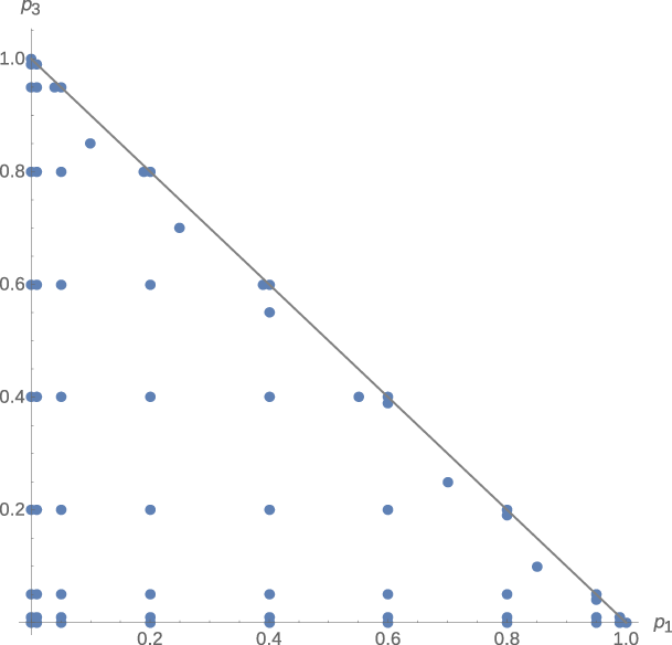
| Figure 2: The Marschak-Machina triangle with the lotteries examined in the
experiment. |
2 Method
The idea of the non-parametric method of plotting
indifference curves comes from contour mapping: a contour line (often
simply called a “contour”) joins points of equal elevation (height) above
a given level, e.g., mean sea level. The procedure is as follows. First,
the lotteries to be examined are chosen; these are the points in the
Marschak-Machina triangle. Second, lottery certainty equivalents (CE) are
determined; these are the “heights” of the respective points. Finally,
these CE values are used to plot a contour map; the contours are the
required indifference curve(s) joining points having the same interpolated
CE value.
2.1 Lotteries involved
The experiment involved 67 lotteries for each of two payoff schedules:
x1 = 0 zł, x2 = 150 zł, x3 = 300 zł (Triangle 1); and x1 = 0
zł, x2 = 450 zł and x3 = 900 zł (Triangle 2). Złoty (zł) is the
Polish currency; $1 ≈ 4 zł, although the purchasing power for
basic goods is closer to identity. Of the 67 lotteries, 3 were located in
the corners of the triangle, 24 on the boundaries, and the remaining 40 in
the interior. To verify the boundary effects, the distribution of lotteries
was chosen to be more dense near the triangle boundaries and corners
(Figure 2).
The lotteries were constructed from the following list of p1 and
p3 probabilities: {0, 0.01, 0.05, 0.2, 0.4, 0.6, 0.8, 0.95, 0.99,
1}. All combinations { p1, 1−p1−p3, p3} such
that 1−p1−p3≥0 resulted in the lotteries: {0, 1, 0}, {0,
0.99, 0.01}, {0, 0.95, 0.05}, etc. The following lotteries were
added to verify the boundary effects close to the hypotenuse: {0.04,
0.01, 0.95}, {0.19, 0.01, 0.8}, {0.39, 0.01, 0.6}, {0.6, 0.01,
0.39}, {0.8, 0.01, 0.19}, {0.95, 0.01, 0.04}, all having p2 =
0.01 and {0.1, 0.05, 0.85}, {0.25, 0.05, 0.7}, {0.4 0.05, 0.55},
{0.55, 0.05, 0.4}, {0.7, 0.05, 0.25}, and {0.85, 0.05, 0.1}, all
having p2 = 0.05.
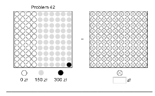
| Figure 3: An example problem from the experiment. |
2.2 CE determination
The term “certainty equivalent” was not used in the instruction (see
Appendix 2), as it is unknown or difficult to understand for most
people. The lotteries were presented in the form of urns containing
black, gray and white balls (for lotteries located in the corners or on
the edges of the triangle, the balls were only one or two colors). To
the right of the urn containing the balls of three colors was another
urn that only contained balls with crosses.
An example problem is demonstrated in Figure 3. In this sample problem,
the value of the black ball was 300 zł, the gray ball 150 zł, and the
white ball 0 zł. The subjects had to state the value that a ball
with a cross would need to have to make them indifferent between
drawing a ball from the left or right urn. The subjects thereby
determined the CEs of the lotteries presented on the left side of the
panel.
The experiment was conducted on the Internet. The problems were presented
to the subjects in random order. Six HTML forms with 134 randomly
ordered problems were prepared. A given form was randomly assigned to each
subject. The black ball offered the maximum payoff in three of the
forms, and the minimum payoff in the others. The gray ball always offered
an intermediate payoff.
2.3 Subjects
There were 237 subjects, all undergraduate economics
students at the Warsaw School of Economics. Their ages ranged from 18 to
25 years with a mean of 20.2 years and 47% were women. The students
received information about the experiment from their supervisors, who
worked with the author of this paper and agreed to promote the
experiment. Participation was voluntary. The subjects were given a
12-zł voucher that they could redeem at the campus cafeteria. As is
known from the literature, the incentive method may have an impact on
the level of risk aversion demonstrated by subjects (e.g., Holt &
Laury, 2002). The subjects were therefore incentivized by
performance as well. They were informed beforehand that some of them
would be taking part in a real lottery. Four subjects were randomly
selected after the data had been collected. The two who offered the
lowest CE for a randomly selected lottery received the amounts they
quoted (70 zł and 90 zł). The other two (who quoted CEs of 100 zł and
130 zł) had to play this lottery. They did not, however, win anything.
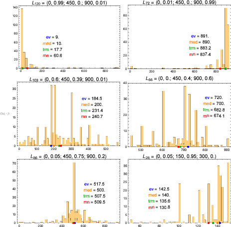
| Figure 4: Example histograms of CE responses for particular lotteries
presented with expected (ev), median (med), mean (mn) and 20% trimmed
mean (trm) values. |
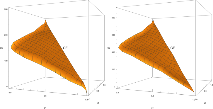
| Figure 5: 3D plots of the aggregated CE values: Triangle 1 (left); and
Triangle 2 (right). |
As the experiment was conducted on the Internet, the subjects could
respond at their convenience. They first registered and familiarized
themselves with the instructions online. They were then required to
solve two sample problems. The time to answer all questions was planned
at 40–50 minutes, although they were asked to work at their own pace.
The average time was about 41 minutes. The value of the voucher (12 zł)
therefore exceeded the minimum hourly wage in Poland, which is about 10
zł.
3 Results
3.1 Aggregating the data
Responses in experiments involving lottery CEs are usually noisy,
skewed, and contain a lot of outliers. The level of noise encountered
in this experiment is probably magnified by the fact that many of the
lotteries under consideration involved three outcomes, rather than two,
as in typical lottery experiments. Moreover, people tend to round their
CE valuations to the nearest ten, fifty, or even hundred (e.g., 10, 50,
700 rather than 9, 54, 670). These rounded CE values may then appear
several times in the responses of different subjects. The term “tied
values” is used in the literature on robust statistics to describe
repetitive responses (see e.g., Wilcox, 2011, 2012). Example histograms
of CE responses obtained for particular lotteries are presented in
Figure 4.
For the reasons presented above, it is of great importance to choose a
proper measure of CE location. The mean value is known to be very
sensitive to outliers (e.g., the upper left graph in Figure 4, which has
a mean value of 60.6, but a median value of only 10.0). The median
value is less sensitive to outliers. However, it is sensitive to tied
values (e.g., graphs in the middle row and the lower left, with a median
of 200, 700, and 500). Many robust location estimators are proposed in
the literature. The trimmed mean estimator is simple to compute, yet,
according to Wilcox (2012), often performs better than more complex
ones when sampling from heavy-tailed distributions. More specifically,
it usually has a narrower confidence interval than the median, mean,
and other measures of central tendency. The trimmed mean is the mean of
the elements in a list after dropping a fraction f of the
smallest and largest elements. Wilcox (2011) suggests f = 20%
for data in social and behavioral sciences. The 20% trimmed mean is a
compromise between the mean (f = 0 %; no points dropped) and
the median (f = 50%; all but one point dropped). Therefore,
as seen in Figure 4, the 20% trimmed mean (in green) assumes a value
between the mean (in red) and the median (in orange).
Applying the 20% trimmed mean estimator results in 134 aggregated CE
values (presented in Appendix 1), which are further used in the
analyses. However, using median or mean CE values does not change the
general observations regarding the shape of the indifferences curves.
3.2 Plotting the CE surfaces
The aggregated CE values are first visualized using a 3D plot (see
Figure 5). Note that the three triangle corners are tied to the values
of 0, 150, and 300 (left) and 0, 450, and 900 (right), as they
represent certainties. Observe the CE surface shape at its edges. The
surface rises and drops sharply at the p1 and p3 axes,
although the slope is maintained at the hypotenuse.
Note that moving upwards from the p1 axis into the area of positive
p3 values (i.e., introducing a new high outcome x3) sharply
increases the lottery CE value. Per contra, moving right from the
p3 axis into the area of positive p1 values (i.e., introducing
a new low outcome x1) sharply decreases the lottery CE value. This
suggests that changing the range of lottery outcomes might explain this
pattern. No such sharp change in the CE value is observed when moving
from the cube diagonal into the triangle interior (i.e., introducing a
new middle outcome x2). In this case, however, the range of lottery
outcomes remains unchanged.
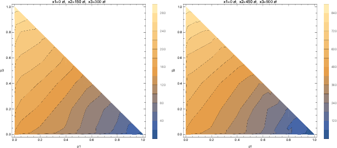
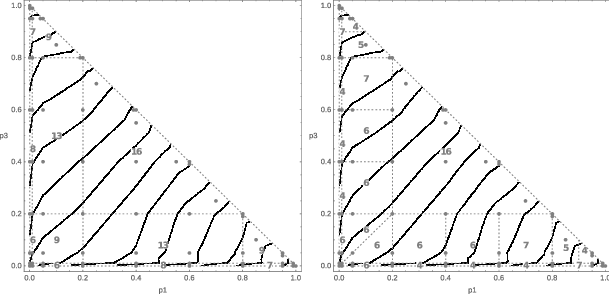
| Figure 6: Indifference curves in two Marschak-Machina triangles: Triangle 1
(left) with outcomes x1 = 0 zł,
x2 = 150 zł, and x3 =
300 zł; and Triangle 2 (right) with outcomes x1
= 0 zł, x2 = 450 zł, and
x3 = 900 zł. The Mathematica®
program draws colored contour plots, so that areas of low CE contour
values are marked using “cold” colors, and areas of high contour values
are marked using “warm” colors. |
3.3 Plotting the indifferences curves
The indifference curves are plotted using the Wolfram
Mathematica® ListContourPlot function, which generates a
contour plot from height values defined at specified points. Similar
functionalities are offered by e.g., “filled.contour” in R and “contour” in
Matlab. According to the Mathematica® tutorial, the
program plots the required contour lines by linearly interpolating heights
along the lines connecting adjacent points on the plane. For instance, to
plot a contour of 200, the program first searches for points on the plane
having an interpolated height of 200. Connecting these points then results
in the required indifference curve of 200. Note that the indifference
curves are plotted using a single command: no dedicated software is
needed. The indifference curves obtained using aggregated CE values for
Triangle 1 and Triangle 2 are shown in Figure 6.
Note that indifference curves are expressed in terms of monetary CE
values, rather than hypothetical “utils” (see plot legends). The
contour values of 0, 20, 40, …., 300 are presented in the left diagram,
and those of 0, 60, 120, …, 900 in the right (which results in 14
curves on each plot). However, the plots for any arbitrarily chosen
number of indifference curves and indifference curve values can be
generated without re-running the experiment.
Several observations need to be made. First, the indifference curves seem
to be straight parallel lines in the middle of the triangle. This is the
area where behavior conforms to Expected Utility Theory.
Second, the further north of the origin towards the northwest corner of
the triangle, the flatter the slopes of the indifference curves, and
the further east of the origin towards the southeast corner of the
triangle, the steeper the slopes of the indifference curves. This
results in a pattern of “fanning-in” around the two legs of the
triangle (i.e., the tendency to intersect at a point to the north-east
of the hypotenuse) and “fanning-out” in the area around the southwest
corner of the triangle (i.e., the tendency to intersect at the point to
the south-west of the origin).
Finally, and most importantly for the present study, the indifference
curves appear to have jumps in the direction of the origin near the
legs of the triangle. Significantly, these jumps are not observed near
the hypotenuse.
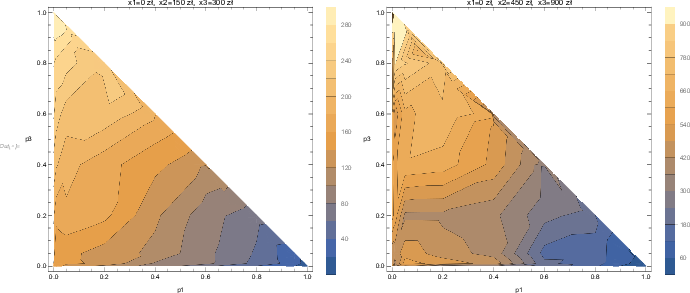
| Figure 7: Simulated indifferences curves after adding a Gaussian noise to
aggregated certainty equivalents. On the left: σ =0.05, on the
right: σ =0.20. |
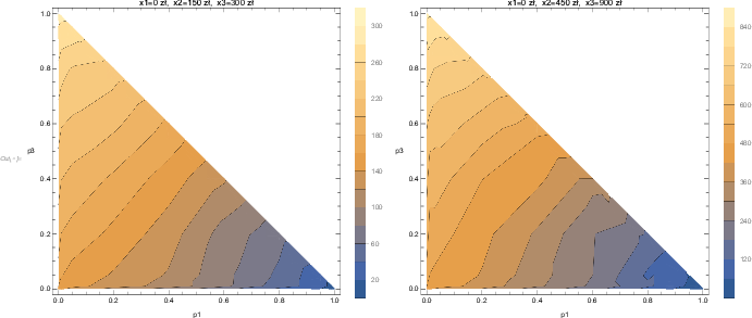
| Figure 8: Simulated indifferences curves after adding a Gaussian noise to
individual certainty equivalents, and then aggregated them using 20%
trimmed mean. On the left: σ =0.05, on the right: σ
=0.20. |
3.4 Limitation and robustness of the method
The method of non-parametrically plotting indifference curves is
sensitive to noise and often results in plots of poor quality when
applied to individual data. At the same time, it is very robust when
the individual data are aggregated using the 20% trimmed mean. The
limitation and the robustness of the method will be illustrated by the
following simulation. Let us assume that the pattern of the
indifference curves presented in Figure 6 reflects the real preferences
of the “average” subject, but a Gaussian noise is added to every
aggregated certainty equivalent value:
C_i^noise=CE_i(1+N(0,σ^2)) .
The simulated indifference curves are presented in Figure 7. As can be
seen, even a small noise ( σ =0.05, graph on the left) seriously
distorts the curves, and a larger one ( σ =0.20, graph on the
right) results in curves that would suggest a lack of any pattern in
the triangle interior and at its boundaries. In fact, the plot on the
right resembles the plots of many of the subjects who took part in the
experiment.
However, adding a Gaussian noise to individual certainty equivalents
(which are already very noisy), and aggregating them using 20% trimmed
means, results in an almost perfect recovery of the observed pattern
(see Figure 8). In fact, there is hardly any discernible difference
between the curves presented in Figure 6 and Figure 8: the median
absolute difference between the certainty equivalent values used to
plot them is 0.4% for σ =0.05 (graphs on the left), and 2%
for σ =0.20 (graphs on the right).
| Figure 9: Sub-areas of the Marschak-Machina triangle used to determine local
slopes of indifference curves. The numbers on the graph show the number
of lotteries in each area. |
The following conclusions can be drawn. First, the method might not be
suitable for plotting individual indifference curves, unless some other
means of reducing the noise are implemented (see also the discussion in
Section ??). Second, the lack of “nice” plots on
the individual level does not necessarily result from a lack of any
interesting effects at the boundaries and in the interior of the
triangle; the method simply fails to recover them when the noise level
is high. Third, the method is very robust when individual data are
aggregated using the 20% trimmed means. Fourth, the pattern obtained
on the group level very likely demonstrates the real preferences of the
“average” decision maker and is not the result of misidentification.
4 Indifference curve slopes
The main observations concerning the shape of
the indifference curves are confirmed by estimating their slopes in the
triangle sub-areas. If decision-makers behave as predicted by
Expected Utility Theory, then their preferences can be represented
in the Marschak-Machina triangle by a set of parallel straight line
indifference curves. For x2=(x1+x3)/2, as in
the present experiment, the slope of the indifference curves for risk
averse people is greater than 1, for risk seeking people less than 1,
and for risk neutral people equal to 1. Lottery CEs may serve to
determine indifference curve slopes using a linear model:
p_3=a+bp_1+cCE ,
in which the required slope is given by the parameter b.
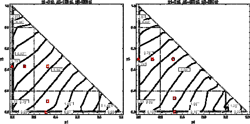
| Figure 10: Indifference curves estimated non-parametrically from the experiment
presented together with local estimations of their slopes in Triangle 1
(left) and Triangle 2 (right). The statistical significance of the
estimated slope values is denoted as: ** for p-value
≤ 0.01, and * for 0.01<p-value ≤
0.05. Area A: 0 ≤ p1 ≤
0.01 and 0.2 ≤ p3 ≤
0.8; Area B: 0.01 ≤ p1
≤ 0.2 and 0.2 ≤ p3
≤ 0.8; Area C: 0.2 ≤ p1
≤ 0.8 and 0.2 ≤ p3
≤ 0.8; Area D: 0.2 ≤ p1
≤ 0.8 and 0.01 ≤ p3
≤ 0.2; Area E: 0.2 ≤ p1
≤ 0.8 and 0 ≤ p3
≤ 0.01. |
4.1 The entire triangle
The minimum least squares procedure applied to aggregated CE values in
the entire triangle leads to b = 1.02 (0.03) for Triangle 1,
and b = 1.06 (0.03) for Triangle 2 (standard errors are given
in parentheses). This suggests that, on average, the subjects
demonstrated slight risk aversion.
4.2 Triangle sub-areas
The same least squares procedure may be applied in triangle sub-areas to
determine local slopes in indifference curves. The triangle has been
split into smaller regions as presented in Figure 9. The numbers on the
graph show the number of lotteries in each area. It is assumed that
lotteries located on the boundaries between two regions (marked as
dotted lines) belong to both regions.
A linear regression procedure was performed in each of these regions to
obtain a number of linear models approximating the indifference curves
locally (the number of degrees of freedom in each model is 3 less than
the number of lotteries). The b value estimations for
aggregated CE values are presented graphically in Figure 10. The
statistical significance of estimated slope values is marked with **
for p-value ≤ 0.01, and * for 0.01 <
p-value < 0.05. Definitions of areas A, B, C, D,
and E, which are most important for deriving conclusions, are given in
Figure 10.
4.3 Areas of straight parallel lines and fanning-in patterns
It can be seen that the indifference curves in Area C of Triangle 1 are
parallel straight lines with a slope of 1.14 (0.04). This is the area
of conformity to Expected Utility.
At the same time, the slope of the indifference curves is 0.87 (0.08) in
Area B, and 1.45 (0.22) in Area D. The same pattern (albeit with some
distortions) can be seen in Triangle 2, where the slope values are 1.00
(0.08), 0.78 (0.12), and 1.60 (0.30) respectively. This indicates a
fanning-in pattern in areas B and D: indifference curves tend to
converge to a point somewhere to the north-east of the Marschak-Machina
triangle.
4.4 Jumps at the legs
These results reveal a sudden change in the slopes of the indifference
curves close to the triangle legs. In Triangle 1, the slope value
changes from 1.45 (0.22) in Area D to 0.07 (0.01) in Area E, i.e., by a
factor of 20. In Triangle 2, there is a similar change from 1.60 (0.30)
to 0.10 (0.02), i.e., by a factor of 16. The same pattern is observed at
the vertical leg. In Triangle 1, the slope value changes from 6.79
(1.90) in Area A to 0.87 (0.08) in Area B, i.e., by a factor of 8, and
in Triangle 2 from 8.79 (2.99) to 0.78 (0.12), i.e., by a factor of 11.
Less abrupt changes can also be observed in the areas around the three
triangle corners, but the results in this case are not statistically
significant.
Unfortunately, the regression procedure on the individual level leads to
statistically insignificant results: individual b values
estimated in the most interesting triangle sub-areas A, B, D, and E
involving 8 or 13 points were statistically insignificant
(p-value > 0.05) for the vast majority of
subjects (93% for Triangle 1, and 95% for Triangle 2). The slope
values estimated for the remaining subjects assumed a value of 1 in
about half the cases, meaning that they gave lottery expected value as
their responses.
4.5 Continuous or discontinuous indifference curves?
These data raise the question as to whether these jumps at the triangle
legs are continuous or discontinuous. It could be argued that 0.01, the
minimum non-zero probability used in the experiment, is still far
greater than 0 (at least on a logarithmic scale) and that the
indifference curves might become smooth for probabilities of less than
0.01. The hypothesis regarding continuity or discontinuity of the
indifference curves at the triangle legs is, however, not testable.
Even if the jumps observed in the experiment had occurred at a
probability of say 0.001, it could still be argued that this was far
greater than 0.
The path of the indifference curves near the two legs of the triangle
suggests, however, that the jumps in the curves are discontinuous. It is
highly unlikely that the indifference curves, which are parallel as they
depart from the hypotenuse and remain so in the middle of the triangle,
would first turn away from the origin, and then (somewhere between a
probability of 0 and 0.01) smoothly turn back towards it. The indifference
curve discontinuity hypothesis would not require such dramatic changes in
the slope values: the indifference curves would remain steep near the
horizontal leg for any non-zero probability p3, and remain flat near the
vertical leg for any non-zero probability p1.
5 Model estimation
The observations presented so far were confirmed
using another analysis: the data collected in the experiment were used to
estimate and compare six decision-making models under risk. Four of them
predict jumps at the triangle boundaries. The idea of this analysis is to
check which models, predicting smooth or discontinuous indifference curves,
better describe the data collected. The models are estimated using CE
values obtained from the experiment and the sum of squared errors (SSE)
values are compared to choose the most accurate model. Certainty
equivalents were used in the past to estimate the CPT parameters (e.g.,
Tversky & Kahneman, 1992; Gonzales & Wu, 1999) and to compare
decision-making models (e.g., Blavatskyy, 2007). This approach differs from
other studies (e.g., Hey & Orme, 1994), in which models were compared on
the basis of preference questions and correct predictions of choices
between two lotteries.
5.1 The models
The typical shapes of the indifferences curves predicted by the models
under consideration are presented in Figure 1. How these models evaluate CE
is detailed below. As before, it is assumed that x1<x2<x3. In what
follows (especially in the case of binary lotteries)
xL=Min[xi] and xH=Max[xi]
will occasionally be used to denote lottery minimum and maximum outcomes
having respective probabilities of pL and pH (when p1=0, the
minimum outcome is x2 rather than x1; when p3=0, the maximum
outcome is x2 rather than x3). A power utility function
v(x)=xα is assumed for the first four models and the
predicted CE value is the utility inverse of the functional.
Expected Utility Theory (EUT, von Neumann and Morgenstern,
1944) is the standard model of decision-making under risk. It evaluates
prospects as follows:
v(CE_EUT)=∑i=1nv(x_i)p_i .
As the model is linear in probabilities, the indifference curves in the
Marschak-Machina triangle are parallel straight lines with no jumps at
the triangle boundaries.
Prospective Reference Theory
(PRT; Viscusi, 1989) is a variant
of the Expected Utility model in which the individual treats stated
probabilities as imperfect information and uses them to update his/her
prior probabilities to posterior ones in the standard Bayesian fashion.
For convenience, the theory assumes a prior probability of 1/n for each
outcome, where n is the number outcomes with pi>0. It follows that:
v(CE_PRT)=β∑i=1nv(x_i)p_i+(1-β)1/n∑i=1nv(x_i) ,
where the parameter β weights: a). the expected utility
functional using stated probabilities (the term on the left) and b).
the expected utility functional using equal probabilities of 1/n
(the term on the right). Changing the number of outcomes n results
in a discontinuous change of the predicted
CEPRT value. This leads to discontinuous jumps
of the indifference curves at all triangle boundaries. As the model is
linear in probabilities, the indifference curves inside the triangle
are parallel straight lines, as they are in the EU model.
Cumulative Prospect Theory
(CPT; Tversky & Kahneman, 1992)
evaluates prospects using a probability weighting function
w(p) applied to cumulative probabilities; the probability
weights are then de-cumulated. Three-outcome lotteries are evaluated using
the functional:
v(CE_CPT) =v(x_3)w(p_3)+v(x_2)[w(p_3+p_2)-w(p_3)]+
v(x_1)[1-w(p_3+p_2)] ,
As the CPT model is nonlinear in probabilities, the indifference curves
in the Marschak-Machina triangle are also nonlinear: they are concave
in the upper-left part of the triangle and convex in the lower-right
part for a typical inverse S-shaped probability weighting function. The
probability weighting function is described in this study using the
two-parameter Prelec (1998) function:
w(p)=e^-γ(-lnp)^δ ,
where parameter δ is responsible for the curvature (lower the
parameter value, more curved the function), and parameter γ
is responsible for the elevation (lower the parameter value, greater
the elevation).
There is no discontinuous change of the predicted
CECPT value when one pi becomes 0, and the
functional simplifies to
v(CECPT)=v(xL)+[v(xH)−v(xL)]w(pH).
Therefore, the indifference curves predicted by the CPT model are smooth
everywhere.
TAX model
(TAX; Birnbaum, 2008) assumes that prospect branches
are assigned decision weights that depend on the “attention” that the
decision maker allocates to a particular branch. A risk-averse
individual shifts attention from high outcome branches to low outcome
ones. The lottery utility is then a weighted average of the outcome
utilities with weights that depend on probabilities and outcome
rankings. Three-outcome lotteries are evaluated as:
v(CE_TAX3)=Av(x_1)+Bv(x_2)+Cv(x_3)/A+B+C ,
where: A=t(p1)+δ /4t(p2)+δ /4t(p3),
B=(1−δ /4)t(p2)+δ /4t(p3), and C=(1−δ /2)t(p3), and where t(p) is the weight
of the branch’s probability (not decumulative probability as in CPT),
and parameter δ defines attention (weights) transfers from
branch to branch (higher the parameter value, greater the attention
transfers to lower branches). Two-outcome lotteries are evaluated as:
v(CE_TAX2)=Av(x_L)+Bv(x_H)/A+B ,
where: A=t(pL)+δ /3t(pH) and
B=(1−δ /3)t(pH). The weights
A, B, and C change discontinuously when the
number of outcomes with a positive probability varies. Therefore, the
lottery valuation changes discontinuously in this case and the
indifference curves might be discontinuous at all triangle boundaries.
The probability weighting function t is described using the power
function t(p)=pγ , and, as the model is nonlinear
in probabilities, the indifference curves are nonlinear: concave in the
left-upper part of the triangle and convex in the lower-right part, as
they are in the CPT model.
Decision Utility model
(DUT; Kontek & Lewandowski, 2018)
applies a normalized utility function D (decision utility) to each
lottery range under consideration. This way the lottery valuation
depends on its range [xL,xH]. Lotteries are compared
with respect to their CE values:
CE_DUT=x_L+(x_H-x_L)D^-1[∑i=1nD(x_i-x_L/x_H-x_L)p_i] .
| Table 1: Estimation results of several decision-making models under
risk. |
| | | | | Parameters |
|
Model | SSE | AIC | BIC | Est. value | St. error | p-value |
| EV | 54 792.9 | 1190.1 | 1195.9 |
| EUT | 54 631.6 | 1189.7 | 1195.5 | α = 0.99 | 0.02 | <10−101 |
| ST | 46 427.1 | 1169.9 | 1178.6 | δ = 0.91 | 0.02 | <10−92 |
| | | | | θ = 20904 | 43400 | 0.63 |
| CPT | 32 118.0 | 1122.5 | 1134.1 | α = 1.12 | 0.05 | <10−46 |
| | | | | γ = 1.09 | 0.04 | <10−52 |
| | | | | δ = 0.86 | 0.01 | <10−96 |
| TAX | 30 183.1 | 1114.2 | 1125.8 | α = 1.05 | 0.02 | <10−83 |
| | | | | γ = 0.95 | 0.02 | <10−73 |
| | | | | δ = 0.12 | 0.02 | <10−5 |
| PRT | 24 860.8 | 1086.2 | 1094.9 | α = 0.96 | 0.01 | <10−124 |
| | | | | β = 0.91 | 0.01 | <10−139 |
| DUT | 20 003.7 | 1057.1 | 1065.8 | r0 = 0.40 | 0.02 | <10−37 |
| | | | | δ = 1.24 | 0.02 | <10−105 |
For a binary lottery, the functional simplifies to:
CEDUT2=xL+(xH−xL)D−1(pH),
which is the same as for CPT, assuming v(x)=x, and
D−1(p)=w(p). Contrary to CPT, however, when
one pi becomes 0 and the lottery range [xL,xH]
changes, the predicted CEDUT value changes
discontinuously. Therefore, the indifference curves are discontinuous
at the triangle legs, but not at the hypotenuse. As the model is linear
in probabilities, the indifference curves inside the triangle are
parallel straight lines, as they are in the EU model. The D
function is described in this study using the CDF of the Two-Sided
Power Distribution (Kotz & van Dorp, 2004):
D(r)={r_0(r/r_0)^δ0<r≤r_0
1-(1-r_0)(1-r/1-r_0)^δr_0<r≤1 ,
where r=xi−xL/xH−xL denotes the relative position of
xi within the lottery range [xL,xH], δ is
the parameter responsible for the curvature (greater the parameter
value, greater the curvature), and r0 defines the value of
r at which the curve crosses the diagonal.
Salience Theory
(ST; Bordalo, Gennaioli & Schleifer, 2012)
provides a context-dependent representation of lotteries in which true
probabilities are replaced by decision weights distorted in favor of
salient payoffs. The functional for the lottery CE is not given in the
original paper and its derivation indicates flaws in the model (for
details, see Kontek, 2016). For instance, the CE value is undefined for
some probability intervals. More seriously, any assumption regarding CE
in those intervals violates monotonicity. Only the formula for binary
lotteries is presented below:
CE_ST={x_L+(x_H-x_L)p/p+δ(1-p)p<δ/δ+A
Ax_L+(A-1)θ/2δ/δ+A<p<1/1+δA
x_L+(x_H-x_L)δp/δp+(1-p)p>1/1+δA ,
where: A=√2xH+θ /2xL+θ , p=pH,
parameter θ affects the salience function σ
(xi,xj)=|xi−xj|/|xi|+|xj|+θ
(greater the parameter value, lower the salience of payoffs in a
given state), parameter δ measures the extent to which
salience distorts decision weights (lower the parameter value, less
salient states are more discounted), and where a constant CE value in
the middle row is assumed to make the model operational. The model
predicts discontinuous jumps at all boundaries, as introducing or
removing an outcome results in a discontinuous change in the predicted
CE value. The indifference curves are non-parallel straight lines
(there are areas of fanning-in, fanning out, and constant CE). Despite
its peculiar features, the ST model is used in this study because it
has recently gained a lot of attention among researchers.
5.2 Estimation results on the group level
The fit of 134 aggregated CE values was performed using the Mathematica
“NonlinearModelFit” function, which constructs a nonlinear least-squares
model and assumes that errors are independent and normally
distributed. Possible settings for the search method include
“ConjugateGradient”, “Gradient”, “LevenbergMarquardt”, “Newton”,
“NMinimize”, and “QuasiNewton”, with the default being “Automatic” (in
which case the method is chosen automatically by the function; this option
was used in estimations). The “NonlinearModelFit” function enables the
parameter space to be constrained, but this was not required for the
aggregate data (except of the ST model). The estimation results are
presented in Table 1. As can be seen, the two-parameter DUT model offers
the best fit, and the PRT model, which also has two parameters, the next
best. The three-parameter TAX model is third, and the CPT model, which also
has 3 parameters, only comes fourth. The ST model, with much poorer
results, is fifth (the p-value of the θ parameter is very high
indicating problems with estimation of the salience function
σ (xi,xj) which is essential for the ST model). The
one-parameter EUT model is only slightly better than Expected Value. This
model ranking is confirmed by the AIC and BIC measures.
As seen the DUT, PRT, and TAX models predicting jumps at the triangle
boundaries are more accurate than CPT, which predicts smooth
indifference curves. This happens even though the DUT and PRT models
use one parameter less than CPT. The poor performance of the ST model
is not surprising given its peculiar features as described above.
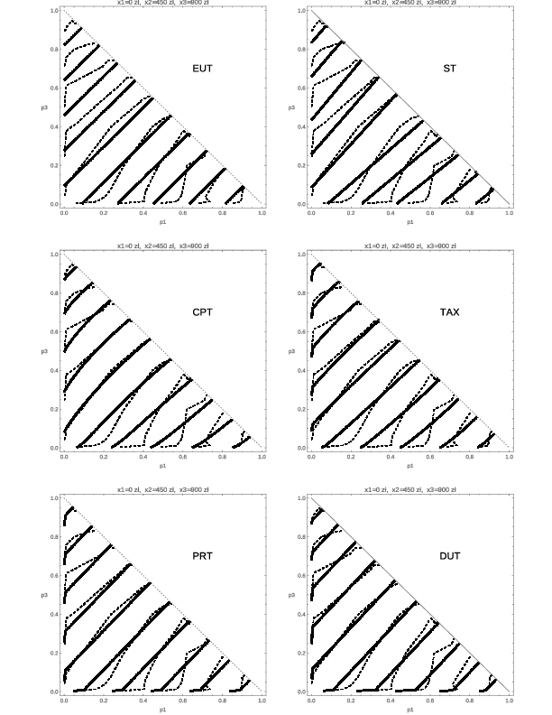
| Figure 11: Indifference curves obtained non-parametrically (dashed) and predicted
by the best-fit models. |
5.3 Predicted vs. observed indifference curves
To make the estimation results more readily comprehensible, the
indifference curves predicted by the best-fit EUT, ST, CPT, TAX, PRT,
and DUT models are presented in Figure 11, together with the
indifference curves obtained non-parametrically. The plots illustrate
the manner and extent to which the predicted curves match those
obtained non-parametrically. As can be seen, the best-fit PRT and DUT
models predict discontinuous jumps on both legs towards the triangle
origin, while the best-fit TAX model predicts discontinuous jumps on
the vertical leg only (jumps at other boundaries are almost invisible).
The CPT model does not predict any jumps. This explains the ranking of
the models obtained in the comparison.
| Table 2: The number of subjects for whom the respective model has the
lowest SSE value. |
| Model | CPT | TAX | PRT | DUT |
| Number of subjects | 110 | 47 | 34 | 46 |
| Percentage of subjects | 46.4% | 19.8% | 14.3% | 19.4% |
These ranking results suggest that the boundary effects at the triangle
legs capture most of the variation in the data. The nonlinearity of the
indifference curves in the triangle interior (if any) is only a
second-order effect. Both the DUT and PRT models perform well because
they conform to Expected Utility inside the triangle, and, at the same
time, capture the specific effects at the triangle legs. Note the
difference between the DUT and PRT models. The size of predicted jumps
along both legs is always the same for PRT but differs for DUT. This
explains why the DUT model performs better than PRT.
It should be noted that the best-fit PRT and TAX models do not predict
any jumps at the hypotenuse, although they generally allow such jumps
(in fact, they predict jumps at the hypotenuse, but these are too small
to be seen on the plot). This additionally confirms that the jumps in
the indifference curves are present only at the triangle legs.
| Table 3: The number
of subjects for whom the respective two-parameter model has the lowest
SSE value. |
| Model | CPT | TAX | PRT | DUT |
| CPT: γ = 1; TAX: γ = 1 | 55 | 47 | 51 | 84 |
| CPT: γ = 1; TAX: β = 1 | 46 | 38 | 65 | 88 |
| CPT: α = 1; TAX: γ = 1 | 77 | 41 | 49 | 70 |
| CPT: α = 1; TAX: β = 1 | 71 | 27 | 61 | 78 |
| Average | 62.25 | 38.25 | 56.5 | 80 |
| Percentage of subjects | 26.3% | 16.1% | 23.8% | 33.8% |
5.4 Estimation results on the individual level
The CPT, TAX, PRT, and DUT models were next estimated using individual
data. Individual data is much more noisy than aggregate data and, in
some cases, may lead to problems with obtaining results. Therefore,
fits were performed with the constrained parameter space (although the
constraints were not too restrictive; for instance, it was assumed for
the CPT model that 0<α <4, 0<γ <20, and 0<δ
<20). Four starting points were chosen for each individual and each
model, and the estimation with the lowest SSE value was chosen as the
best fit. Calculations were performed with the working precision of 16
digits and were conducted in parallel using 8 Mathematica kernels.
The most accurate model for each subject (i.e., having the lowest SSE
value), was then chosen. Table 2 shows the number of subjects for whom
the respective model was the most accurate.
| Table 4: The number of subjects for whom the two-parameter CPT or DUT
model has a lower SSE value, and the mean and median absolute
differences between the models expressed in
%. |
| The best model | CPT | DUT | Mean absolute difference in SSE | Median
absolute difference in SSE |
| CPT: γ =1 | 96 (40.5%) | 141 (59.5%) | 5.3% | 3.6% |
| CPT: α =1 | 115 (48.5%) | 122 (51.5%) | 5.8% | 3.8% |
As can be seen, the CPT model has the lowest SSE value for 46.4% of
subjects. Other models, which allow jumps in the indifference curves at
the triangle boundaries, are the best in the case of the remaining
53.6%. As the CPT and TAX models have three parameters, whereas PRT
and DUT only two, estimations were also made for two-parameter versions
of the CPT and TAX models to make the comparison fair. In the case of
CPT, the version with γ = 1 means that a nonlinear value
function was used together with a one-parameter probability weighting
function, and the version with α =1 means that a linear
value function was used together with a two-parameter weighting
function. In both cases, the two-parameter CPT model performs poorer
than previously, and the DUT model becomes the prevailing one for
33.8% of subjects on average (see Table 3).
Importantly, the CPT model, which predicts smooth indifference curves,
is, on average, the best for only 26.3% of subjects (20-33% depending
on which two parameters are used). Other models (including DUT), that
allow jumps in the indifference curves at the triangle boundaries, are
the best for the remaining 73.7%. The PRT model is generally slightly
less accurate than CPT on the individual level, and the TAX model is
the worst in this comparison.
A direct comparison was finally made between the two-parameter versions
of the CPT and the DUT models. In this case, DUT offers more accurate
fits for 51.5%-59.5% of subjects and performs slightly better than
CPT. The results are presented in Table 4.
It may be argued that the model comparisons presented in Tables 2, 3,
and 4 identify a discrete “winning model”. An SSE difference of 0.01
could lead one to claim that one model is superior without any way to
determine the difference between this situation and one where a model
excels by a difference of 100. Therefore, Table 4 presents also mean
and median absolute differences between the models in terms of SSE
(calculated as an average for all individuals). As seen, the best model
fits differ on average by 5.3%-5.8% (from 0.1% to 363%) in terms of
SSE with either CPT more accurate than DUT, or DUT more accurate than
CPT. This shows that either one or another model offers a clear
advantage for a given individual.
The analysis of individual data presented in this section confirms the
existence of the boundary effects captured by models that predict jumps
at the triangle legs. The comparison also shows that the CPT model
performs comparatively better on the individual than on the aggregate
level. The flexibility of this model by the addition of the third
parameter (important when individual data diverge from the average
pattern) may explain this result.
6 Related literature
Many studies have tested the various hypotheses
about the shape of the indifference map (e.g., Hey & Strazzera, 1989,
Camerer, 1989; Loomes, 1991; Harless, 1992; Harless & Camerer, 1994;
Abdellaoui & Munier, 1998; Blavatskyy, 2006; Bardsley et al., 2010).
There are generally two ways to identify indifference curves in
experiments: ask indifference questions; ask preference questions. The
former involves asking subjects to indicate those lotteries to which
they are indifferent vis-à-vis a given one. This procedure allows an
indifference curve to be plotted by connecting the points representing
indifferent lotteries inside the triangle (Hey & Strazzera, 1989).
The method proposed in this paper is a version of this general
approach: subjects indicate certainty equivalents to which they are
indifferent vis-à-vis a given lottery, and these certainty equivalents
serve to plot the indifference curves. The other approach involves
presenting subjects with a set of pairwise choices and asking them to
indicate their preferences (e.g., Harless & Camerer, 1994). This
approach allows only hypotheses regarding the shapes of indifference
curves in the triangle or regions of it to be tested. Combinations of
both approaches have been used. Loomes (1991) and Cubitt et al. (2015)
ask indifference questions to test hypotheses about the shapes of
indifference curves and underlying axioms. Yet another approach is used
by Hey and Orme (1994), who ask preference questions to estimate
preference functionals (i.e., decision-making models). The indifference
curves predicted by the best model indicate the underlying pattern.
The observation that the EU model works fine for lotteries inside the
Marschak-Machina triangle has often been reported in the literature.
Hey and Orme (1994) state that the EU model appears to fit no worse
than any of the other models for 39% of subjects. Similarly, Carbone
and Hey (1994) find that approximately half their subjects appear to
conform to the EU model. Hey and Strazzera (1989) additionally find
that, for the majority of their subjects, the indifference curves were
in accordance with EU theory. Abdellaoui and Munier (1998) find that
the shape of the indifference curve is compatible with the EU
hypothesis along the middle part of the hypotenuse and in the
“immediate” interior of that middle part. This result is very close to
the one obtained in the present study.
The existence of fanning-in has been reported in the literature by e.g.
Hey and Di Cagno (1990), who observed that the fanning-in point was to
the northeast of one of the three triangles for 14 subjects. Moreover,
the indifference curves fan in for 22 of the 56 subject/triangle pairs.
Blavatskyy (2006) presents a more detailed study concerning
“fanning-out” and “fanning-in”, and suggests that an individual’s
indifference curves tend to “fan-in” when probability mass is
associated with the best and the worst outcomes and tend to “fan-out”
when probability mass is associated with intermediate outcomes. The
results presented in this paper are clearly close to Blavatskyy’s
summary.
There is evidence of boundary effects in the literature, although how
and to what extent these effects affect the shape of the indifference
curves is not clearly stated. Conlisk (1989) moved the Allais lotteries
to the interior of the triangle and concluded that EU theory violations
are less frequent and cease to be systematic when boundary effects are
removed. Camerer (1989), Harless (1992), and Sopher and Gigliotti
(1993) obtained similar results. Harless and Camerer (1994), after
analyzing a large number of experimental data sets, conclude that the
EU model should be used when all the lotteries have the same number of
probable outcomes (i.e., the lotteries are located in the interior of
the triangle), but a different model has to be used when the lotteries
have different numbers of probable outcomes (i.e., some of the lotteries
are located on the boundaries or in the corners of the triangle).
Boundary effects were studied in detail by Abdellaoui and Munier
(1998), who concluded that indifference curves were distorted near
triangle boundaries. They draw a distinction, however, between behavior
near different edges of the triangle. One test, restricted to segments
linking the hypotenuse to the triangle interior leads to an acceptance
of the hypothesis of parallelism. By contrast, the same hypothesis
concerning the segments linking the left and lower edges to the
interior is strongly rejected. The present experiment not only captures
this difference but additionally shows that the distortion near the
triangle legs is due to jumps towards the triangle origin in the
indifference curves.
7 Optimal lottery grid
It may be argued that the variability of the
indifference curves at the triangle legs observed in the present
experiment (coupled with a lack of such variability in the triangle
interior) is simply the result of repeated measurements in this region
of the triangle. The jumps, so this reasoning goes, are observed at the
legs because that is where the points were repeatedly sampled; had
several points been measured close to any point in the triangle
interior, similar jumps would have been observed. This objection can be
easily countered by stating that, if the variability at the legs is the
result of repeated sampling, then the variability observed at the
hypotenuse, where the measurement points were likewise densely located,
should be similar. This, however, is not the case.
More broadly, this objection raises an important question concerning the
optimal lottery grid in Marschak-Machina triangle experiments. It is
well known from experiments involving binary lotteries that the
greatest variability in lottery certainty equivalents occurs for
probabilities close to 0 and 1: the change of the certainty equivalent
value is large when the probability changes from 0 to 0.01, or from 1
to 0.99, but not that large when the probability changes from 0.50 to
0.51. This phenomenon is best expressed by an inverse S-shaped
probability weighting function (Tversky & Kahneman, 1992; Gonzales
& Wu, 1999), which is nonlinear at the probability endpoints and
almost linear in the middle. Tversky and Kahneman (1992) offered a
psychological hypothesis to explain this shape, which they called
diminishing sensitivity. According to this hypothesis, people become
less sensitive to changes in probability as they move away from 0 or 1,
just as they are less sensitive to changes in outcome values as they
move away from the reference point.
It follows that the optimal set of lotteries to test diminishing
sensitivity experimentally should consist of more lotteries having
probabilities close to 0 and 1. Therefore, Tversky and Kahneman used
lotteries having probabilities of 0.01, 0.05, 0.10, 0.25, 0.50, 0.75,
0.90, 0.95, and 0.99, rather than having an equal spread. The
diminishing sensitivity observed experimentally is thus not the result
of applying more lotteries close to the probability endpoints, but
certainly more lotteries at the probability endpoints are required to
test the anticipated diminishing sensitivity (for a contrary opinion
see Stewart, Reimers & Harris, 2015). For the very same reason, and
in order to verify the boundary effects, the distribution of lotteries
in the Marschak-Machina triangle in the present study was chosen to be
more dense near the triangle boundaries and corners. Using
probabilities having an equal spread could make any boundary effects
impossible to detect. Note that some previous investigations were
conducted using an equal spread of probabilities (e.g., Hey & Orme,
1994, with a spread of 1/8). It is therefore not surprising that the
EU model appeared to fit no worse than any of the other models for a
substantial percentage of subjects, as the boundary effects had not
been probably taken into account in the experimental set-up. This also
applies to the present data: removing lotteries close to the triangle
boundaries (i.e., having probabilities of either 0.01 or 0.05) from the
data set results in plots of the indifference curves showing no jumps
at the legs.
Verifying whether there is any local variability in the triangle
interior would require more lotteries in this region. This would
resemble detailed testing of the probability weighting function shape
around its middle part, which, according to many studies, is more less
linear. Thus, although such examination is possible, it would probably
result in conclusions stated already in this paper and in a number of
former studies, i.e., that the indifference curves in the middle part of
the Marschak-Machina triangle are linear with local variability caused
possibly by the noise only.
The question of how to select an optimal lottery grid inside the
Marschak-Machina triangle not only involves determining the shape of
the indifference curves, but also estimating the model parameters, and
comparing decision-making models. The model estimation results
presented in this paper come with the caveat that the fits and the
model ranking apply only to the specific lottery grid in the
Marschak-Machina triangle examined in the experiment. The grid used in
the experiment involves many lotteries in the vicinity of the triangle
edges (to explore the boundary effects), so the model ranking could be
quite different for a different grid. In fact, removing lotteries close
to the triangle boundaries from the data set results in CPT having the
highest ranking, followed by DUT, TAX, and PRT. On the other hand,
using a grid with an equal probability spread would possibly lead to a
ranking that does not take any boundary effects into account, even so
well accepted in the literature as overweighting of small probabilities
and underweighting of large ones. This raises the general question of
how to select an optimal lottery grid when discriminating between
decision-making models (Cavagnaro et al., 2013). Designing an optimal
lottery grid based on axioms in order to plot the indifference curves
and to discriminate between the models of decision-making under risk is
certainly an interesting direction of future research. The number of
lotteries used in the experiment is one of the parameters that needs to
be optimized: the natural inclination to increase this number would
lead to more detailed plots, but, on the other hand, would leave the
subjects less time to focus on each problem and would probably
increase the noise. Thus limiting, rather than increasing the number of
lotteries should be also considered.
8 Discussion
This paper presents experimental results
concerning the shape of indifference curves in the Marschak-Machina
triangle. The plots obtained non-parametrically indicate that: (i)
indifference curves are straight parallel lines in the middle part of
the triangle; this is the area of conformity to the Expected Utility
model; (ii) the indifference curves “fan-in” along the triangle legs
(but not in their vicinity); and (iii) the indifference curves jump
towards the origin along the two legs of the triangle; these boundary
effects are, however, not present at the hypotenuse. This observation
is confirmed by estimating the slopes of the indifference curves in the
triangle sub-areas and by estimating six decision-making models under
risk.
The model ranking naturally leads to a discussion on which of the
psychological phenomena underlying the models best explains the shape
of the indifference curves obtained in this study. The path of the
indifference curves near the two legs of the triangle suggests that the
jumps in the curves are discontinuous. Abrupt changes in the slopes of
the indifference curves were statistically confirmed in the vicinity
of both triangle legs. The discontinuity of indifference curves is not
particularly welcomed by mathematicians and could even be regarded as a
weakness in the model. One possible explanation of this phenomenon
could be discontinuity in probabilities. This feature has a solid
psychological foundation and is prevalent in the psychological
literature. The tendency to overweight certain outcomes relative to
merely probable ones was labeled the “certainty effect” by Kahneman and
Tversky (1979). Certain outcomes, however, are located in the corners
of the Marschak-Machina triangle, and only the jumps starting from
there can be explained by this effect. Discontinuity in decision
weights for probabilities close to 0 and 1 is a slightly more general
concept which can also be applied to lotteries located on the triangle
boundaries. This holds, however, for all probabilities, including the
probability of the middle outcome. The indifference curves are
therefore discontinuous at all three triangle boundaries in the
original Prospect Theory.
Cumulative Prospect Theory, per contra, predicts smooth indifference
curves. For this reason, they do not match the indifference curves obtained
in this study particularly well. Moreover, the lottery certainty
equivalents (especially their aggregated values) are not fitted so
accurately by CPT as by other models. This raises the question as to
whether the cumulative probability weighting postulated by CPT is the right
phenomenon to explain the anomalies observed in decision-making under
conditions of risk. The original idea of probability weighting applied to
individual probabilities (Kahneman & Tversky, 1979) was simple and
convincing: small probabilities are overweighted whereas medium and large
ones are underweighted. Unfortunately, this kind of probability weighting
violates first-order stochastic dominance, which limits its applicability
to prospects involving no more than two non-zero outcomes. Weighting of
cumulative probabilities was introduced to fix this issue (Quiggin, 1980;
Yaari, 1989; CPT, Tversky & Kahneman, 1992). This solution is
mathematically elegant and allows prospects involving any number of
outcomes to be considered. Psychologically, however, it is less plausible,
as this would mean that people assess probabilities cumulatively rather
than individually. Birnbaum (2004) has presented evidence to refute this.
The results presented in this study provide further evidence that the
cumulative probability weighting postulated by CPT might not be
psychologically vindicated.
The phenomenon of range dependence (Parducci, 1965; Cohen, 1992; Kontek &
Lewandowski, 2018) is sound psychologically and adequately explains the
pattern observed. Introducing a new high outcome x3 results in an upward
payoff range extension and a sharp increase in the lottery CE
value. Introducing a new low outcome x1 results in a downward payoff
range extension and a sharp decrease in the lottery CE value. Introducing
a new middle outcome x2 does not change the payoff range and so no sharp
change in the lottery CE value is observed. Essentially, the same
explanation was presented earlier by Abdellaoui and Munier (1998):
lotteries located on the legs of the triangle do not have the same support
as those located elsewhere in the triangle; as a result, either p1=0 or
p3=0 implies a more dramatic change in individual behavior than
p2=0. The three-criteria1 (Cohen,
1992) and decision utility (Kontek & Lewandowski, 2018) models, both
based on range dependence, predict parallel straight line indifference
curves in the triangle interior with jumps towards the triangle origin at
the legs. This pattern was stated non-parametrically in the present
study. The DUT model was, moreover, the most accurate in fitting aggregated
certainty equivalents and in fitting individual ones when two-parametric
models were compared.
Prospective Reference Theory (Viscusi, 1989) predicts the same pattern
of the indifference curves as models based on range dependence, but
allows jumps at the hypotenuse. These happened to be almost invisible
for the aggregated data and the fit was only slightly less accurate
than that of DUT. The PRT model was slightly less accurate than CPT on
the individual level. It is interesting to note that the PRT model was
also among the winners in Hey and Orme’s study (1994). Its good
performance in this study is therefore not accidental. However, the
assumption underlying the theory that individuals treat stated
experimental probabilities as imperfect information and use them to
update their prior probabilities to posterior ones in the standard
Bayesian fashion, seems psychologically less plausible.
Models founded on other psychological phenomena only partially explain
the shape of the indifference curves obtained in this study. The TAX
model, which postulates a shift in attention from high outcome branches
to low outcome ones, generally predicts various shapes of the
indifference curves with jumps allowed at all boundaries. However, the
shape predicted by the best-fit model only partially corresponds with
the stated one (jumps on the vertical axis only). As a result, the
model takes an intermediate position in the rankings: it performs
better than CPT on the group level, but does not perform so well on the
individual level. The overweighting of salient outcomes postulated by
Salience Theory has recently gained a lot of attention among
researchers as a phenomenon explaining anomalies in various areas of
economics and finance. The shape of the indifferences curves predicted
by this model is, however, in strong disagreement with the one stated
in this study. As a result, the Salience Theory model fits the lottery
certainty equivalents collected in the experiment poorly and performs
only slightly better than EU.
To sum up, the best lottery certainty equivalent fits were offered by
models that predict parallel straight line indifference curves in the
triangle interior with jumps at the legs towards the origin. The shape of
the indifference curves obtained non-parametrically explains this
result. As stated in previous studies, Expected Utility Theory generally
holds in the triangle interior. This study shows that the psychological
phenomenon of range-dependence best explains the boundary effects. To
conclude, Expected Utility holds for lotteries having the same range of
outcomes; Expected Utility is violated when the range of outcomes changes
(note that the lotteries in the famous Allais paradox have different
ranges).
The above analysis was made possible thanks to a novel method of
plotting indifference curves inside the Marschak-Machina triangle using
lottery certainty equivalents. One major advantage of this method is
that it allows the indifference curves to be visualized, and not merely
hypotheses concerning their shapes to be tested. Moreover, plots can be
obtained using a standard command available on most statistical
packages, without any dedicated software having to be written.
One problem encountered in this study is the high level of noise
observed in the certainty equivalent values. The level of noise is
probably magnified by the fact that many of the lotteries under
consideration involved three outcomes, rather than two, as in typical
experiments. Despite this, the method proposed generates clear
indifference curve patterns for individual data aggregated using 20%
trimmed means, and is very robust, even if the noise level in
individual responses is artificially increased, as shown by a separate
simulation. The method, however, results in poor quality plots when the
level of noise is too high. Therefore, it often fails to demonstrate a
clear pattern of individual indifference curves, which exposes its
limitation. Possible approaches towards solving this problem include
conducting similar experiments in a laboratory, rather than on the
Internet, using stronger incentive schemes, and devising other ways of
determining certainty equivalents. It is not certain, however, whether
using these means will result in cleaner data. A better approach might
be to repeat collecting responses from the same subject. This would
allow his/her responses to be averaged and the noise levels at given
measurement points to be reduced. Another option would be to perform a
smoothing procedure on the plane in order to get the average value of
the points in the vicinity of any given one. The initial tests using a
smoothing procedure demonstrated the advantage of this approach and, in
many cases, a great improvement of the plots quality. However, care
needs to be exercised when smoothing values on the plane as it may also
smooth the jumps, which are of the greatest interest in this study.
References
Abdellaoui, M., Munier, B. (1998). The Risk-structure Dependence Effect:
Experimenting with an Eye to Decision-aiding. Annals of
Operations Research, 80, 237–252.
Bardsley, N., Cubbit, R., Loomes, G., Moffat P., Starmer C., & Sugden R.
(2010). Experimental Economics: Rethinking the Rules. Princeton
University Press.
Becker, J. L., & Sarin, R. K. (1987). Lottery Dependent Utility.
Management Science, 33(11), 1367–1382.
Birnbaum, M. H. (2004). Tests of rank-dependent utility and cumulative
prospect theory in gambles represented by natural frequencies: Effects
of format, event framing, and branch splitting. Organizational
Behavior and Human Decision Processes, 95, 40–65.
Birnbaum, M. H. (2008). New paradoxes of risky decision making.
Psychological Review, 115, 463–501.
Blavatskyy, P. (2006). Axiomatization of a Preference for Most Probable
Winner. Theory and Decision, 60, 17–33.
Blavatskyy, P. R. (2007). Stochastic expected utility theory.
Journal of Risk and Uncertainty, 34(3), 259–286.
Bordalo, P., Gennaioli, N., & Schleifer, A. (2012). Salience theory of
choice under risk. The Quarterly Journal of Economics, 127(3),
1243–1285.
Camerer, C., (1989). An experimental test of several generalized
utility theories. Journal of Risk and Uncertainty, 2,
61–104.
Carbone, E., & Hey, J. D. (1994). Estimation of expected utility and
non-expected utility preference functionals using complete ranking data. In
Munier B., & Machina M. J. (Eds.) Models and experiments in risk
and rationality, pp. 119–139 Kluwer Academic Publishers.
Cavagnaro, D., Gonzales, R., Myung, J. I., & Pitt, M. A. (2013). Optimal
Decision Stimuli for Risky Choice Experiments: An Adaptive Approach.
Management Science, 59(2), 358–375.
Chew, S. H., MacCrimmon, K. (1979). Alpha-nu choice theory: A
generalization of expected utility theory. Working paper 669,
University of British Columbia.
Cohen, M. (1992). Security level, potential level, expected utility: A
three-criteria decision model under risk. Theory and Decision,
33(2), 101–134.
Conlisk, J., (1989). Three variants on the Allais example.
American Economic Review, 79(3), 392–407.
Cubitt, R. P., Navarro-Martinez, D., & Starmer, C. (2015). On preference
imprecision. Journal of Risk and Uncertainty, 50(1),
1–34.
Dekel, E. (1986). An axiomatic characterization of preferences under
uncertainty: Weakening the independence axiom. Journal of
Economic Theory, 40, 304–318.
Gonzales, R., & Wu, G. (1999). On the shape of the probability weighting
function. Cognitive Psychology, 38, 129–166.
Gul, F. (1991). A Theory of disappointment aversion.
Econometrica, 59, 667–686.
Harless, D. (1992). Predictions about indifference curves inside the
unit triangle. Journal of Economic Behavior and Organization,
18, 391–414.
Harless, W., & Camerer, C. (1994). The predictive utility of generalized
expected utility theories. Econometrica, 62(6),
1251–1289.
Hey, J. D., & Strazzera E., (1989). Estimation of indifference curves in
the Marschak-Machina triangle. Journal of Behavioral Decision
Making, 2, 239–260.
Hey, J. D., & Di Cagno, D. (1990). Circles and triangles: An experimental
estimation of indifference lines in the Marschak-Machina triangle.
Journal of Behavioral Decision Making, 3, 279–306.
Hey, J. D., & Orme, C. (1994). Investigating generalizations of expected
utility theory using experimental data. Econometrica,
62(6), 1291–1326.
Holt, C. A., & Laury, S. K. (2002). Risk aversion and incentive effects.
American Economic Review, 92(5), 1644–1655.
Jia, J., Dyer, J. S., & Butler, J. C. (2001). Generalized disappointment
models. Journal of Risk and Uncertainty, 22(1),
59–78.
Kahneman, D., & Tversky, A. (1979). Prospect theory: An analysis of
decision under risk. Econometrica, 47(2), 263–291.
Kontek, K. (2016). A critical note on Salience Theory of choice under
risk. Economics Letters, 149, 168–171.
Kontek, K., & Lewandowski, M. (2018). Range-dependent utility.
Management Science, 64(6), 2812–2832.
Kotz, S., & van Dorp, J. (2004). Beyond beta. Other continuous families of
distributions with bounded support and applications. World
Scientific Publishing.
Lopes, L. L. (1987). Between hope and fear: The psychology of risk.
Advances in Experimental Social Psychology, 20,
255–295.
Loomes, G., & Sugden, R. Regret theory: An alternative theory of rational
choice under uncertainty. Economic Journal, 92,
805–824.
Loomes, G. (1991). Testing decision theories by using ‘value
equivalences’. Oxford Economic Papers, 43, 644–666.
Machina, M. (1982). Expected utility analysis without the independence
axiom. Econometrica, 50, 277–323.
Marschak, J. (1950). Rational behavior, uncertain prospects, and
measurable utility. Econometrica, 18(2), 111–141.
Neilson, W. S. (1992). Some mixed results on boundary effects.
Economics Letters, 39, 275–278.
Parducci, A. (1965). Category judgment: A range-frequency model.
Psychological Review, 72(6), 407–418.
Prelec, D. (1998). The probability weighting function.
Econometrica, 66, 497–527.
Quiggin, J. (1982). A theory of anticipated utility. Journal of
Economic Behavior and Organization, 3(4), 323–43.
Sopher, B., & Gigliotti, G. (1993). A test of generalized expected utility
theory. Theory and Decision, 35, 75–106.
Stewart, N., Reimers, S., & Harris, A. J. L. (2015). On the origin of
utility, weighting, and discounting functions: How they get their
shapes and how to change their shapes. Management
Science, 61(3), 687–705.
Tversky, A., & Kahneman, D. (1992). Advances in prospect theory:
Cumulative representation of uncertainty. Journal of Risk and
Uncertainty, 5, 297–323.
Viscusi, K. (1989). Prospective reference theory: Toward an explanation
of the paradoxes. Journal of Risk and Uncertainty, 2,
235–264.
Von Neumann L. J., & Morgenstern, O. (1944). Theory of games and economic
behavior. Princeton University Press, Princeton, NJ.
Wilcox, R. (2011). Modern statistics for the social and behavioral
sciences: A practical introduction. CRC Press, Taylor & Francis Group,
Boca Raton, FL.
Wilcox, R. (2012). Introduction to robust estimation and hypothesis
testing. Elsevier.
Yaari, M. E. (1987). The dual theory of choice under risk.
Econometrica, 55(1), 95–115.
Appendix 1: CE values aggregated for the group for Triangle 1
(CE300 column) and Triangle 2 (CE900 column).
| P1 | p2 | p3 | CE300 | CE900 |
| 0 | 0 | 1 | 300.0 | 900.0 |
| 0 | 0.01 | 0.99 | 294.2 | 886.3 |
| 0 | 0.05 | 0.95 | 278.7 | 842.6 |
| 0 | 0.2 | 0.8 | 259.4 | 778.8 |
| 0 | 0.4 | 0.6 | 228.7 | 682.8 |
| 0 | 0.6 | 0.4 | 209.4 | 625.3 |
| 0 | 0.8 | 0.2 | 188.8 | 558.8 |
| 0 | 0.95 | 0.05 | 172.3 | 499.4 |
| 0 | 0.99 | 0.01 | 158.9 | 466.4 |
| 0 | 1 | 0 | 150.0 | 450.0 |
| 0.01 | 0 | 0.99 | 292.1 | 883.2 |
| 0.01 | 0.04 | 0.95 | 274.8 | 838.2 |
| 0.01 | 0.19 | 0.8 | 250.5 | 759.4 |
| 0.01 | 0.39 | 0.6 | 222.6 | 648.9 |
| 0.01 | 0.59 | 0.4 | 201.0 | 579.0 |
| 0.01 | 0.79 | 0.2 | 180.5 | 524.2 |
| 0.01 | 0.94 | 0.05 | 161.0 | 477.2 |
| 0.01 | 0.98 | 0.01 | 150.2 | 451.1 |
| 0.01 | 0.99 | 0 | 146.5 | 442.0 |
| 0.04 | 0.01 | 0.95 | 272.5 | 819.0 |
| 0.05 | 0 | 0.95 | 273.8 | 831.6 |
| 0.05 | 0.15 | 0.8 | 238.4 | 737.0 |
| 0.05 | 0.35 | 0.6 | 217.5 | 639.2 |
| 0.05 | 0.55 | 0.4 | 193.5 | 570.8 |
| 0.05 | 0.75 | 0.2 | 172.8 | 507.5 |
| 0.05 | 0.9 | 0.05 | 152.1 | 456.0 |
| 0.05 | 0.94 | 0.01 | 145.9 | 436.9 |
| 0.05 | 0.95 | 0 | 135.6 | 411.6 |
| 0.19 | 0.01 | 0.8 | 229.9 | 699.9 |
| 0.2 | 0 | 0.8 | 230.8 | 705.6 |
| 0.2 | 0.2 | 0.6 | 205.9 | 599.6 |
| 0.2 | 0.4 | 0.4 | 178.3 | 506.3 |
| 0.2 | 0.6 | 0.2 | 155.3 | 446.6 |
| 0.2 | 0.75 | 0.05 | 138.2 | 417.1 |
| P1 | p2 | p3 | CE300 | CE900 |
| 0.2 | 0.79 | 0.01 | 132.5 | 400.1 |
| 0.2 | 0.8 | 0 | 113.7 | 362.5 |
| 0.39 | 0.01 | 0.6 | 178.3 | 525.5 |
| 0.4 | 0 | 0.6 | 176.5 | 522.0 |
| 0.4 | 0.2 | 0.4 | 151.0 | 425.7 |
| 0.4 | 0.4 | 0.2 | 127.9 | 374.4 |
| 0.4 | 0.55 | 0.05 | 118.4 | 330.8 |
| 0.4 | 0.59 | 0.01 | 111.3 | 328.9 |
| 0.4 | 0.6 | 0 | 92.1 | 277.4 |
| 0.6 | 0 | 0.4 | 121.1 | 365.0 |
| 0.6 | 0.01 | 0.39 | 121.0 | 333.9 |
| 0.6 | 0.2 | 0.2 | 92.3 | 255.0 |
| 0.6 | 0.35 | 0.05 | 84.6 | 244.0 |
| 0.6 | 0.39 | 0.01 | 85.0 | 231.4 |
| 0.6 | 0.4 | 0 | 66.8 | 204.0 |
| 0.8 | 0 | 0.2 | 66.8 | 172.4 |
| 0.8 | 0.01 | 0.19 | 66.5 | 169.8 |
| 0.8 | 0.15 | 0.05 | 55.9 | 111.9 |
| 0.8 | 0.19 | 0.01 | 49.9 | 131.4 |
| 0.8 | 0.2 | 0 | 36.6 | 104.8 |
| 0.95 | 0 | 0.05 | 31.1 | 54.3 |
| 0.95 | 0.01 | 0.04 | 28.8 | 57.4 |
| 0.95 | 0.04 | 0.01 | 29.7 | 50.3 |
| 0.95 | 0.05 | 0 | 21.0 | 36.0 |
| 0.99 | 0 | 0.01 | 13.1 | 17.7 |
| 0.99 | 0.01 | 0 | 9.0 | 16.5 |
| 1 | 0 | 0 | 0 | 0 |
| 0.1 | 0.05 | 0.85 | 251.6 | 760.8 |
| 0.25 | 0.05 | 0.7 | 210.5 | 618.0 |
| 0.4 | 0.05 | 0.55 | 172.9 | 495.3 |
| 0.55 | 0.05 | 0.4 | 127.9 | 373.9 |
| 0.7 | 0.05 | 0.25 | 87.4 | 253.1 |
| 0.85 | 0.05 | 0.1 | 46.5 | 108.1 |
Appendix 2 – Instruction (a translation from Polish)
The left and right urns each have 100 balls. You are required to select
a ball at random from one of the two urns.
The left urn has black, white and gray balls. The value of each ball is
given under the illustration. Selecting a ball from this urn carries a
risk. The payoff depends on the color of the ball and its value.
All the balls in the right urn are marked with a cross. They are all
identical. Therefore, if you select a ball from this urn, you are
guaranteed a given sum of money with absolutely no risk.
Task:
Nominate the value of the balls in the right urn that would make you
indifferent between a random selection from either urn, i.e., so that it
would not matter to you which urn you chose when making a random
selection.
Example 1:
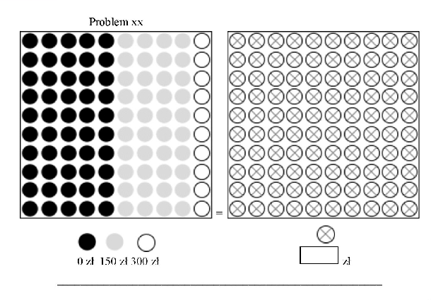
In this example, the left urn has 50 black balls with a value of 0 zł,
40 gray balls with a value of 150 zł, and 10 white balls with a value
of 300 zł.
a) Think of the value a cross-marked ball would need to have to make you
indifferent as to which urn to choose when selecting a ball at random.
Write this value under the right illustration.
b) If you feel that you would prefer to select a ball from the right
urn, then the value you have nominated for the cross-marked balls is
too high.
c) If you feel that you would prefer to select a ball from the left urn,
then the value you have selected for the cross-marked balls is too low.
d) Repeat steps a), b), c) and d) until you are indifferent as to
whether you randomly select a ball from the left or right urn.
Further comments:
Carefully consider the amounts given in the problems, and remember that
you stand to gain real money. In fact, some of you will be selected and
will take part in a real lottery after the experiment is finished.
Try to nominate the value of the cross-marked balls as precisely as
possible – at least to within 5-20 zł. Avoid giving rounded amounts.
The more precise your answers, the greater their academic worth.
Do not try to be “mathematically correct”. Obviously, you are not
prohibited from counting. It might even be advisable that you do so.
Keep in mind, however, that this is a psychological, and not a
mathematical, test.
Verifying the responses
If when completing the next problem, you find a filled-in field changes
color to red, then that field has been filled in incorrectly.
A figure greater than the maximum value of the balls in the left urn
(300 zł in the above example) or less than their minimum value (0 zł in
the above example), or perhaps a non-numerical character, might have
been entered. Your form will not be accepted unless the error is
corrected.
Green, on the other hand, means that the field has been filled in
correctly.
Before you complete the experiment, try one more example.
Example 2:
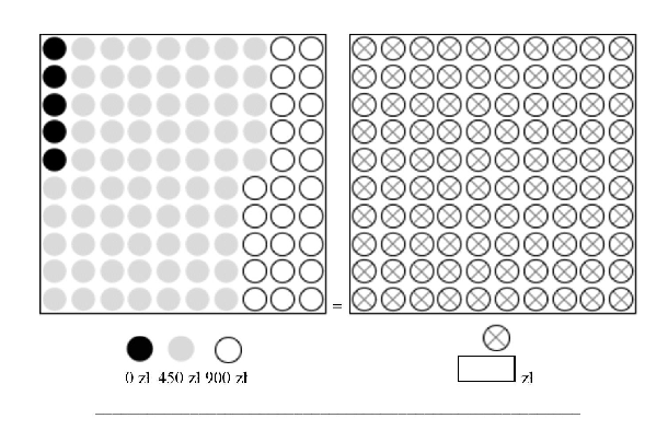
If you understand the instructions, start the test by clicking “Next”.
If you are not sure about anything, read the instructions again.
If you do not wish to complete the test, press “Return”.
This document was translated from LATEX by
HEVEA.