Judgment and Decision Making, Vol. 10, No. 5, September 2015, pp. 469-478

We present a novel method of judgment analysis called Error Parsing, based upon an alternative method of implementing Social Judgment Theory (SJT). SJT and Error Parsing both posit the same three components of error in human judgment: error due to noise, error due to cue weighting, and error due to inconsistency. In that sense, the broad theory and framework are the same. However, SJT and Error Parsing were developed to answer different questions, and thus use different methodological approaches in the analysis of error. While SJT makes use of correlational methods, Error Parsing uses absolute differences. We discuss the similarities and differences between the methodologies and provide empirical evidence for the utility of the Error Parsing technique.
Keywords: Social Judgment Theory, judgment, error.

1  Introduction

In the absence of perfectly predictive cues—a condition that describes nearly every aspect of the world—error in judgment is inevitable. The amount of error, however, depends on any number of factors (e.g., time constraints, number and quality of cues, etc.). Understanding these factors has been a central goal for decision scholars in the interest of both designi ng interventions to reduce error and discriminating amongst different accounts of the cognitive processes underlying human reasoning. However, error has primarily been viewed as a uniform construct; aside from considering the difference between overestimation and underestimation (i.e., Type I and Type II errors), researchers have rarely attempted to parse error into its component parts.

One significant exception to this trend stems from Social Judgment Theory (SJT), an adaptation of Brunswik’s (1952) Lens Model, which has emerged as a popular method of analyzing decision making and providing feedback to judges on how to improve their performance. (For a broad review of Brunswik’s key works, see Hammond & Stewart, 2001.) In this paper, we describe Error Parsing: a novel method of implementing SJT, which we argue can, under the right circumstances, provide a more useful approach to describing the sources of judgment error. The approach is particularly useful when examining real world judgments, as opposed to abstract concepts measured using an arbitrary scale. This paper describes the similarities and differences between Error Parsing and SJT, and empirically illustrates the benefits of using Error Parsing.

1.1  Probabilistic functionalism and the Lens Model

The approach of probabilistic functionalism (Brunswik, 1952) presents humans as “intuitive statisticians” and although it was initially developed in relation to perception, it has been extended from perception to the domain of judgment analysis. Three major principles emerged from Brunswik’s theory. First, Brunswik posited that both the environment in which an individual resides (the ecology) and the individual itself ought to receive equal emphasis and treatment in theory and research (Brunswik, 1955). Second, Brunswik argued that the cues available in any situation would never be perfectly valid or reliable indicators of a construct of interest. He allowed for the fact that cues would often be correlated with one another and thus, possibly redundant, further complicating the decision environment. The third basic principle of probabilistic functionalism is that the available cues would display only a probabilistic relationship to the responses produced by the individual. Because of this, there is uncertainty not only within the ecology but also in how the individual utilizes the cue information. Brunswik argued that these two distinct sources of uncertainty should be described similarly, and used correlational statistics to represent this uncertainty.

---

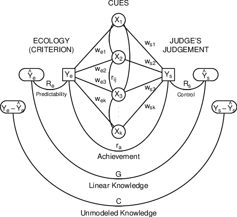
Figure 1: Adaptation of Lens Model for the constructs of SJT.

---

1.2  Social Judgment Theory (SJT)

The broad applicability of the Lens Model outside of visual perception led researchers to extend it to the study of human social judgment (Hammond, 1955). The adapted Lens Model (Figure 1) shows the major constructs of Social Judgment Theory. (For an extensive review of the elements of the Lens Model and SJT, see Hammond et al., 1975 and Cooksey, 1996.)

In SJT, the performance of a judge is measured by the relationships between the validity of the available cues, performance, and consistency of the individual using these cues. There are four key constructs to note in this model. First, on the side describing the ecology, predictability (R_e) describes the relationship between the outcomes (Y_e) and available cues (Ŷ_e). As the cues become noisier and thus less predictive, R_e will decrease. On the side describing the judge, control (R_s) describes the relationship between the predictions made (Y_s) and the way the judge weights the cues (Ŷ_s). As the judge becomes less consistent in how s/he uses the cues, R_s will decrease. Linear knowledge (G) describes the relationship between the model created using the cues (Ŷ_e) and the model based on the weights applied by the judge (Ŷ_s). As the judge pays less attention to predictive information and more attention to unpredictive information, G will decrease. However, G is also based on intercorrelations between the cues, and this can have a larger impact than the judge’s weights. Finally, achievement (r_a) describes the relationship between the actual values (Y_e) and the predictions made by the judge (Y_s). To the extent that the judge is less accurate in his/her overall predictions, r_a will decrease. Each of these relationships is measured by a correlation, allowing them all to be compared and quantified in the same terms, as prescribed by Brunswik’s original theory.

Hammond (1955) initially applied the Lens Model to an examination of the prediction of intelligence quotient (IQ) by clinical psychologists, based upon the results of Rorschach tests. Since then SJT has been used as a tool for judgment analysis in a variety of contexts. For example, SJT has been used to analyze interpersonal conflicts that arise due to cognitive differences (Brehmer, 1976), and in the context of weather forecasting (Stewart, 1990). Researchers have used the principles of SJT to help managers and policymakers understand their own mental processes in a specific choice environment and thus improve their judgments and decisions. The use of SJT has also been proposed as a method of analyzing educational policies and decision making, at both a micro (teacher estimates of student potential) and macro (promotion policies of promotion committee members) level (Cooksey & Freebody, 1986). In all of these examples, the key contribution of SJT is the provision of a quantitative method of analyzing decisions made by individuals or groups by providing insights into aspects of their judgments. This analysis provides a potential tool for intervening in judgment, training experts, and encouraging learning in a dynamic choice environment.

1.3  Bootstrapping individual judgments

At the same time that Hammond and colleagues were promoting the use of probabilistic functionalism to evaluate social judgment, a separate group of researchers were arguing for the use of statistical prediction completely in lieu of clinical prediction. Meehl (1954) originally argued that normative actuarial judgment (i.e., judgment as predicted by statistical models) is far more accurate than expert prediction. A large body of literature has confirmed that human judgment is often less accurate than the output of even the simplest actuarial models. (See Dawes et al., 1989, for a review.) This is perhaps best illustrated by what is known as bootstrapping—a method of improving judgments by replacing predictions made by a human judge with predictions based upon a simplified actuarial model of those judgments. A bootstrap model computes the regression weights of an individual, based on the available cues, and applies those weights consistently to a new set of judgments. In nearly all cases, the bootstrap of an individual will outperform the individual (Dawes & Corrigan, 1974).¹

There are two primary reasons that actuarial models reliably outperform human judges. The first is that people often improperly assign weights to the different cues. While a regression model can take into account every past instance (i.e., the temperature each day since statistics have been recorded) in calculating the optimal weight (β) for each cue (e.g., the barometric pressure or month of the year), humans don’t have the cognitive capacity to engage in such calculations (Simon, 1955). Indeed, a large and varied literature on heuristics has demonstrated that people tend to use cues and strategies that diverge from optimal weighting (for a review, see Shah & Oppenheimer, 2008). However, on its own, inappropriate weighting of cues does not entirely account for the superiority of actuarial models, bootstrapped models in particular (which use the same weights as the judges). Humans are also inconsistent in their use of information. The same objective information presented multiple times is often used differently each time. Since this variance is primarily random error, the more inconsistent a person is when making judgments, the more inaccurate those judgments will be (Camerer, 1981; Dawes, 1971). Even experts are inconsistent in cue selection and weighting, and are not able to equal the accuracy of their bootstraps (e.g., Ashton, 2000). Inconsistency can be such a large source of error that linear models in which all cues are equally weighted, or even randomly weighted, frequently make more accurate predictions than human judges (Dawes, 1979).

---

Figure 2: Graphical representation of the components of error in Error Parsing.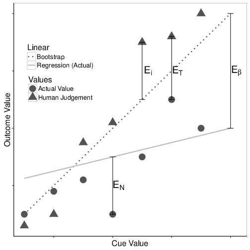

---

In addition to the two sources of human error described above, there is a third type of error that human judges and actuarial models share: noise. That is, the inherent error present in all judgments because no set of cues perfectly predicts every outcome. For example, barometric pressure, season, and previous day’s temperature cannot be combined in such a way as to perfectly predict the next day’s weather. While the amount of noise is dependent on the quality of the cues, virtually no prediction is completely noise free. Finally, it should be noted that error may also arise not only from improper cue weights, inconsistency, or noise, but also from the use of the incorrect cue function forms.²

1.4  Error Parsing

Error Parsing brings together components of probabilistic functionalism and bootstrapping to provide a novel method of implementing SJT. Consider Figure 2, which plots a linear relationship between a hypothetical predictive cue and the outcome to be predicted.

For simplicity, we assume a straightforward linear relationship between the available cues (we discuss other possible function forms later). We define the outcome on a given trial to be O (gray diamonds), the prediction from the regression as R (solid gray line), the prediction from a bootstrap as B (dashed black line), and the human prediction as P (black squares). For the purpose of illustration, Figure 2 has been simplified to represent only a single cue predicting the outcome, however the technique described below works in a multidimensional space (i.e., in the presence of multiple predictive cues) as well.

Total human error (E_T): E_T = |O − P| (1)

The total error of human judgment can be calculated as the absolute difference between the values that an individual predicted, and the actual outcomes (Equation 1). In Figure 2, this difference is represented by the distance between the black squares and the gray diamonds. The better the individual is at making predictions, the closer the actual values will fall to the predicted values. This error is related to the construct of achievement in SJT.³ It is critical to note that this construct ignores the value of directionality in judgment error.

Error due to noise (e_n): e_n = |O − R| (2)

This is the naturally occurring error that results from the fact that predictor variables cannot perfectly predict outcomes even when weighted optimally. As a simplifying assumption, we will consider only linear regressions as the definition of optimal prediction (although the procedure could be applied to non-linear relationships as well). This component can be calculated by taking the absolute difference between the predictions of the optimal model and the actual values of the outcomes (Equation 2). On Figure 2, this is represented by the distance between the gray diamonds and the solid gray line. The better the predictors are, the closer the actual values will fall to their regression line. The error due to noise is related to the construct of optimal predictability in SJT.

Error due to cue weighting (e_β): e_β= |R − B| (3)

This error results from the fact that an individual may not know the appropriate weight to place on the available cues, or may lack the cognitive capacity to use all of the available cues (for a discussion of when people fail to make use of all the informative cues, see Payne, Bettman & Johnson, 1993). Calculating e_β requires one to first construct a model of the performance of the judge. A bootstrap for an individual is constructed by the regression of the cues onto an individual’s predictions. That is, just as a normal regression calculates the optimal weights for predicting outcomes, a bootstrap determines the optimal weights for predicting a human’s predictions. The use of this technique creates the necessary model, or “paramorphic representation” of the individual’s judgment (as described by Hoffman, 1960).

Error due to cue weighting is then calculated as the absolute difference between the prediction of the bootstrap and the prediction of the optimal model (Equation 3), i.e., the difference between the average weight the human places on each cue and the optimal weight that ought to be placed on each cue. On Figure 2, this is represented by the distance between the solid gray line and the dashed black line. Error due to cue weighting would almost exclusively come from errors in knowledge of the prediction domain: the better an individual knows/applies the appropriate weights, the closer these two lines will fall to each other. Error due to cue weighting is related to linear knowledge in SJT.

Error due to inconsistency (e_i): e_i = |P − B| (4)

This error results from the fact that humans are inconsistent in their application of weights to cues. This component can be calculated by taking the absolute difference between the individual’s predicted values and the predictions of the bootstrap model of that individual (Equation 4). That is, inconsistency is captured by the difference between a person’s average cue weighting and the person’s cue weighting on a particular trial. In Figure 2, this is represented as the distance between the black squares and the dashed black line. The more consistent an individual becomes in his/her predictions, the closer the human predictions will come to the bootstrap line. This is related to the construct of cognitive control in SJT.

---

Figure 3: Hypothetical scenario of judges with identical correlation, but different magnitude of error in judgment. SJT would report that the judges have similar error due to this correlation, but the Error Parsing analysis shows that Judge 1 has a greater magnitude of error.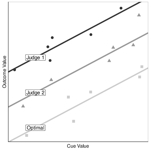

---

1.5  Benefits of Error Parsing

Both Error Parsing and more traditional methods of implementing analyses in SJT rely on the same major constructs. However, while SJT analyses traditionally rely on correlational methods, the use of absolute differences in Error Parsing provides a novel way of examining and providing feedback on judgment. The primary benefit of the Error Parsing technique is that it allows for an examination of the magnitude of error present in judgment. Using the standard correlational approaches of SJT, this is not possible; different amounts of errors can yield identical correlation coefficients if there are differences in the y-intercept, and these differences would be intrinsic to the particular judge. (But see Stewart & Lusk, 1994, for a correlational treatment of SJT that accounts for differences in y-intercepts.) Statistically, a high correlation could be the result of any magnitude of error. Figure 3 provides a hypothetical example of this.

In this case, both judges have identical correlations with the actual values. However, Judge 1 has a much greater magnitude of total error. This difference cannot be observed using standard SJT methods, but is immediately evident when using Error Parsing. The ability to determine the magnitude of error makes it possible to compare the relative amounts of error generated by each component. Specifically, we describe the errors present in the predictions of one judge, based on the validity of the available cues (in the simplified case—for demonstration purposes—of linear relationships between the cues and the outcomes).

We are not the first to identify these problems with correlational methods in SJT. Of particular note is the work of Stewart and Lusk (1994), who went beyond traditional assumptions that increasing the amount and quality of information is all that is needed to improve judgments and predictions. Stewart and Lusk (1994) combine properties of three distinct systems to provide a coherent decomposition of forecasting performance into seven distinct components. They build upon previous research to map this decomposition onto the Lens Model equation to create an expanded Lens Model that accounts for the seven components. The components include: the environmental predictability of available cues, the dependability of the information system, the match between the judge and the environment, and the reliability of both information acquisition and processing. In addition, they describe two types of bias that measure the calibration of forecasts (one based on the mean forecasts and outcomes, the other based on standard deviations). Finally, they discuss examples from the literature that address each component, along with describing implications for analyzing and improving judgments. In other words, Stewart and Lusk identify the biases brought about by correlational methods (such as the y-intercept problems) and then measure and report the extent of those biases as additional components of error.

The related literature on mean absolute error (MAPE) describes a common alternate technique that some researchers prefer to use to describe error. (See Armstrong and Overton, 1977; Armstrong, 1978; Armstrong, 2001.) This measure of prediction accuracy typically expresses a judge’s performance as a percentage. However, this method is biased towards methods with forecasts that are too low (Tofallis, 2014). There are alternate ways to implement MAPE, but they do not give decomposition of error in the way that both SJT and Error Parsing provide. Our research adds to the literature on SJT by further exploring the nuances of the way that error in judgment can be decomposed.

While the aforementioned work is a major advance, it still relies of correlations rather than absolute magnitude of error (as used in Error Parsing). The advantage of being able to identify magnitude of error becomes evident upon comparing data analyzed using each technique, as demonstrated in the experiment and analyses described below.

2  Experiment 1

In some situations, individuals make more accurate predictions when fewer cues are available for consideration (e.g., Arkes, Dawes & Christensen, 1986; Hall, Ariss & Todorov, 2007). A meta-analysis provides further support for the idea that more cues may reduce the quality of judgment (Karelaia & Hogarth, 2008). These effects are counterintuitive because the presence of additional information is nearly always beneficial for statistical models. For this reason, this phenomenon seemed an ideal testing ground for Error Parsing. Although providing additional cues reduces error due to noise, overall error can be greater. Application of Error Parsing can provide insight into which of the other components of error is increasing.

2.1  Participants

A total of 109 participants completed the task on Amazon Mechanical Turk. All participants were United States residents, and there were no requirements for knowledge in the prediction domain. Because of this, participants were provided with brief descriptions of each of the cues (described in more detail below), and we did not measure relative levels of expertise between the judges. Each individual was compensated $1 for completing the task.

2.2  Materials

Two prediction sets were created for this experiment. To ensure ecological validity of the prediction sets, data was sampled from two real world domains (baseball scoring and car blue-book value). In the baseball domain, 25 baseball games were randomly sampled from the 2014 Major League Baseball (MLB) season. The number of hits allowed, walks issued, and strikeouts by a pitcher predicted the number of runs allowed by a pitcher with cue validities of .80, .14 and –.03, respectively. In the blue-book value domain, 25 used cars for sale were randomly sampled from Craigslist. The car’s initial value, the age of the car, and total mileage predicted a car’s current value with cue validities of .40, –.74, and –.78 respectively. The cue validities were the correlations between the cues and the outcomes values.⁴

2.3  Design and procedure

---

Table 1: Analysis of prediction using EP.

Error Type	Symbol	2 cues baseball	3 cues baseball	2 cues blue book	3 cues blue book
Noise	en (Re)	1.05	1.00	$1984	$1972
Improper weighting	eβ (G)	1.48	2.72	$3638	$5149
Inconsistency	ei (Rs)	.66	2.61	$1530	$3217
Total Error	ET (ra)	1.95	1.83	$3542	$3998
Intercept		–.16	.43	$13986	$8876
Note. The components of absolute error do not sum to the total error, because total error is the sum of the signed error, which may cancel. The labels in parentheses indicate the analogous constructs in SJT.

---

---

Table 2: Analysis of prediction using SJT.

Error Type	Symbol	2 cues baseball	3 cues baseball	2 cues blue book	3 cues blue book
Noise	en (Re)	.35	.34	.19	.19
Improper weighting	eβ (G)	.11	.17	.10	.32
Inconsistency	ei (Rs)	.20	.27	.38	.28
Regression bias		.23	.21	.32	.19
Base rate bias		.83	.67	.23	.21
Total Error	ET (ra)	.54	.57	.35	.45
Note. The labels in parentheses indicate the analogous constructs in SJT. Errors in SJT are defined as (1−r2), where r designates the correlation between the appropriate constructs.

---

For each prediction set there were two blocks of trials. In one block participants were given the two most valid cues and asked to predict the outcome for each of the 25 items in the prediction set. In the other block, the same participants were given the same prediction set only with all three cues. The order of the items within each prediction set was randomized, and participants were led to believe that the second set of judgments was being made on a different sample. The order of both the prediction set and the order of the blocks were randomized, and feedback was not provided at any point during the task. Because of the combination of randomized order of presentation of cues between the 2- and 3-cue conditions and the randomization of domain presentation, we did not include order as a factor for analysis. Participants were given the definitions of each cue, and made 50 predictions in each of the two domains (25 with two cues, 25 with three cues) for a total of 100 predictions overall.⁵

To compute the error using Error Parsing, the optimal weighting was calculated using the unstandardized regression coefficients, and these weights were then used to compute the optimal individual predictions for each case using the available cues. The same technique was completed to find each judge’s individual weighting, and the subsequent bootstrapped values. Then, the appropriate differences were taken (absolute values) to find the total error, error due to noise, error due to inappropriate cue weighting, and error due to inconsistency. This process was completed for each individual judge (although the optimal values are the same across participants) and then the error was averaged across judges to compute the results displayed in Table 1. For the SJT analysis, the correlation was found between the analogous terms for each component, and the error was reported as 1−r², as is standard for SJT analysis. These values were averaged across participants to find the values reported in Table 2.

2.4  Results

2.4.1  Effect of adding cues

Replicating the results of previous studies showing that more information can be detrimental to judgment (e.g., Arkes, Dawes & Christenson, 1986; Hall, Ariss & Todorov, 2007), both Error Parsing and SJT indicated that judgments were more accurate in the blue book domain when participants had fewer cues at their disposal. Total error increased from $3,542 in the 2-cue condition to $3,998 in the 3-cue conditions (paired sample t(97) = 1.89, p = .06). SJT also suggests that participants were more accurate in the 2-cue condition (paired sample t(97) = 3.95, p < .01). However, Error Parsing and SJT diverge in the analysis of the baseball condition. Error Parsing suggest that participants were more accurate in the condition with 3 cues (mean total error 1.83 runs) than in the 2-cue condition (mean total error 1.95 runs, paired sample t(99) = 1.92, p = .06). Using the SJT technique, participants appear to be more accurate in the 2-cue condition (paired sample t(97) = 2.10, p = .04). That is, while estimates were more highly correlated with the correct values when participants were shown two cues, the absolute amount of error was smaller when they were shown three cues.

2.4.2  Breaking down the error within condition

There were four experimental conditions in this study: 2-cue-baseball, 3-cue-baseball, 2-cue-bluebook, and 3-cue-bluebook. One way of analyzing the data is to examine how error was distributed within these conditions. While there are certainly instances in which Error Parsing and SJT agree as to the relative magnitude of error, in the discussion below we will highlight the cases where Error Parsing and SJT reveal different stories about the nature of the error. (But see Tables 1 and 2 for a full summary.)

In the 2-cue-baseball condition an Error Parsing analysis suggests that error due to weighting was the largest source of error (mean = 1.48 runs), and contributed more than twice as much error as error due to inconsistency (mean = .66 runs) (paired sample t(99) = 6.67, p < .01). However, an SJT analysis suggests exactly the opposite—with error due to inconsistency (mean = .20) nearly twice as large as error due to weighting (mean = .11), a significant difference (paired sample t(97) = 4.22, p < .01).

In the 3-cue-baseball condition Error Parsing analysis suggests that error due to noise is the smallest source of error (mean = 1.0) while the other two sources of error are more than twice as large (means = 2.72 and 2.61). Both of these are significantly larger than the error due to noise (one-sample t(99) = 6.60, p < .01 and one sample t(99) = 5.37, p < .01; respectively). Meanwhile, SJT analysis suggest that noise is the largest source of error (mean = .34) and nearly twice as large as error due to weighting (mean = .18), one sample t(97) = 6.85, p <.01.

In the 2-cue-bluebook condition, Error Parsing suggests that error due to improper weighting (mean = $3638) is more than twice as large as error due to inconsistency (mean = $1530), a significant difference (paired sample t(97) = 9.88, p < .01). However, SJT suggests the exact opposite—that error due to inconsistency (mean = .38) is massively larger than error due to improper weighting (mean = .10), and this difference is also significant (paired sample t(97) = 14.24, p < .01).

Error Parsing and SJT yield very similar results for the 3-cue-bluebook condition. As the purpose of this study is to highlight differences between the methods, we will go no deeper into this condition except to note that this serves as evidence that the methods do not necessarily diverge. That is, they are different, but not opposing.

2.5  Breaking down error between conditions

Adding an extra cue can change the amount of error (as discussed above) but also the nature of that error. In the baseball domain, SJT and Error Parsing suggest similar stories for what happens to the different types of errors with the addition of a third cue (noise goes down, and weighting and inconsistency go up). While the magnitudes of these changes vary somewhat depending on the method of analysis used, the two methods are largely in agreement.

However, in the bluebook domain, Error Parsing leads to starkly different conclusions than SJT. Error Parsing reveals that the error due to inconsistency more than doubles when a third cue is added (2-cues = $1,530, 3-cues = $3,217; although this difference is not significant (paired sample t(97) = 1.37, p =.17). SJT, on the other hand, suggests that the error due to inconsistency actually decreases (2-cues = .38, 3-cues = .28; (paired sample t(97) = 4.36, p < .01). Once again, SJT and Error Parsing yield very different interpretations of the data.

3  Discussion

3.1  Applications of Error Parsing

Error Parsing provides a significant extension to the judgment analysis literature. First, as demonstrated by the experimental data, in certain cases Error Parsing allows for a clearer analysis of the magnitude of error present in judgment. When analyzing judgments using correlations, the difference in magnitude of the error components can be obscured. As shown in Figure 3, predictions of different judges might show similar correlations with outcomes in a prediction domain, despite vastly different amounts of total error. Figure 3 provides an extreme example of this, but more subtle applications of this logic can explain why SJT and Error Parsing can appear to produce contradictory results. For example, one can imagine a scenario where two judges produce a set of predictions that fall around the proper optimal pattern of judgments. However, one judge could predict a greater distance from these optimal values, on average, causing each judge to have the same correlation with the actual outcomes, but different magnitudes of error. Consider that {1,1 ,1, -1, –1, –1} correlates perfectly with both {1, 1, 1, –1, –1, –1} and {2, 2, 2, –2, –2, –2}. Even though they both have a y-intercept of 0, the absolute average difference is 0 for the first and 1 for the second. Error Parsing would pick up on this subtlety, while SJT would not.

We acknowledge that we are not the first to discuss these problems. As previously discussed, a notable alternative formulation—the Extended Lens Model (Stewart & Lusk, 1994)—proposes a solution that decomposes the performance score of individuals even further, to produce nuanced terms that reflect other sources of bias. This is a very clever solution that, like Error Parsing, both solves the problem of the y-intercept, and accounts for magnitude biases. However, this model still produces analysis of judgment based on correlations, which can obscure the absolute magnitude of the difference, and potentially makes feedback more difficult to interpret and utilize.

What this means is that SJT and Error Parsing are differentially effective depending on the type of question that is being asked. Correlation (and thus SJT) is more appropriate when trying to reduce deviation from ordinal rankings of options, while Error Parsing is better suited to reducing absolute differences. For example, in baseball, SJT is more appropriate if you are trying to determine which pitcher to put into your starting rotation (where you care about the rank order of who will allow the most runs) while Error Parsing would be better for betting on the total number of runs scored in the game (where you care about the absolute error in the number of runs scored).

Even when the two methods yield results in the same direction, Error Parsing allows for clearer inferences about relative contributions of the different components of error. The SJT methodology is harder to interpret; because the error values can be so similar, differences in magnitude can be harder to interpret. Error Parsing allows for the components of error to be compared in a meaningful way, and it makes the magnitude of error observable.

Especially for people who lack expertise in statistics, providing feedback in the form of correlation coefficients may be difficult for judges to interpret and incorporate into subsequent predictions. Feedback in correlations is likely to be more confusing than feedback in the unit of judgment. Feedback in the form of dollars or runs scored is both understandable to laypeople and easily integrated into future judgments. This kind of feedback could help an individual decide upon a more effective prediction strategy. For example, if the judge learned that most error came from inappropriate cue weighting, an intervention might involve training the judge on the relative values of the cues. Meanwhile, if the error primarily came from inconsistency, an intervention might focus on reducing the idiosyncrasies in judgment from trial to trial. Ultimately, to design interventions that address the actual source of error, it is first necessary to be able to accurately break down error into its component parts and understand those component parts.

To the extent that Error Parsing does provide more effective feedback, it could lead the field to reinterpret previous findings. For example, previous research has shown that providing information about cue relationships can improve judgments, but that information about the judge’s perceptions does not (for a review, see Balzer et al., 1989). Because this literature utilizes the methods of social judgment theory, such conclusions may be due to the limitations of the feedback that correlation-based methods provide. Future research could investigate whether Error Parsing provides more effective feedback to judges, and whether it yields different results.

Of course, the relative effectiveness of providing feedback using Error Parsing versus the Extended Lens Model is inherently an empirical question. Further research should directly compare how the provision of feedback to judges through either Error Parsing of the Extended Lens Model might improve judgment.

Despite these scenarios where Error Parsing offers a potential advantage, we note that methods stemming from the Lens Model may be linked to an early tendency to study judgment using abstract scales (e.g., Likert scales). When analyzing judgments that use these types of scales for judgment and feedback, Error Parsing is not the ideal method; when using abstract scales, the notion of absolute differences is often meaningless. However, when attempting to find practical applications of these techniques, the scales being used will have meaning, and so the use of differences may add value, as discussed here, beyond using correlations only.

There are other cases where SJT’s correlational approach would be a more appropriate measure of decision performance as well. For example, when comparing individuals between different judgment domains, absolute differences would not be meaningful—one cannot easily compare $100 dollars to .2 runs. In this case, correlations would allow for a standard unit of comparisons between judges. However, even in these cases, Error Parsing outputs could be provided in ways that allow for such comparisons (such as transforming the absolute error into “percent of average value”). Another approach would be to examine Z-scores for predictions across different domains, which would also provide a meaningful mode of comparison.

3.2  Extensions and future directions

To date, we have considered only simple linear regressions as the definition of optimal prediction. We recognize that this assumption ignores the possibility of interactions among cues, and of curvilinear relationships between cues and outcomes. Previous work has shown that information gathered from linear models sometimes obscures subtle strategies in judgment (such as shifting attention between cues). More nuanced knowledge about judge behavior could help determine which model is better, and could also address more complex judgment patterns such as complete omission of cues or interactions among individual cues.

There have been previous efforts made to address the issue of non-linear relationships between cues, from an SJT approach (see Brannick & Brannick, 1989). It will be worthwhile, in future studies, to explore how Error Parsing can be useful at providing feedback on the magnitude of error using different functions of how cues relate to each other. For example, a non-linear bootstrap of a judge could be created within the Error Parsing methodology, creating a better model of the judge without losing the advantages that this approach offers.

In addition, judges may alter their judgment policies over time. If predicting an exceptionally large number of cases, judges may become fatigued and subtly change the way they utilize the set of available cues. Because Error Parsing averages over a large set of judgments, this change would not be captured in the analysis. However, we note that this shift in prediction patterns would not be observed using standard SJT analysis either.

It is also possible that the problem of cue redundancy may need to be addressed in some scenarios (see Shah & Oppenheimer, 2011). Error Parsing could be adjusted and studied further to explore how it ought to deal with issues relating to multicollinearity and non-linear relationships among cues and outcomes, but that is beyond the scope of this paper. This could be accomplished through both analysis and simulation, to better explore and describe when Error Parsing would provide results distinct from those of SJT.

3.3  Conclusion

Error Parsing provides an extension to previous research exploring techniques for the investigation of error in judgment and prediction. Parsing the sources of error in prediction and judgment can help develop interventions that improve accuracy and facilitate learning. This possibility has implications for judgments such as medical diagnosis and treatment, courtroom punishment and sentencing, and stock market evaluations. Judgment and prediction are ubiquitous and often very important, and tools with the potential to increase accuracy have broad implications. Error Parsing takes the insights derived from the technique of bootstrapping and combines it with the insights of SJT to provide an alternate method to analyze judgment. Future research should continue to compare and contrast alternative techniques to allow for a clearer description of the circumstances under which each provides the most utility.

References

*

Daniel J. Evans School of Public Policy and Governance, University of Washington, Box 353055, Seattle, WA 98195. Email: hallcc@uw.edu.

#

University of California, Los Angeles.

We thank Ryan P. Scott for help with the graphics.

Copyright: © 2015. The authors license this article under the terms of the Creative Commons Attribution 3.0 License.

1

However, it should be noted that, even though bootstrapping can be an effective way of improving judgments, a meta-analysis has shown that the benefit of the method is diminished when judges have some prior experience in the domain of judgment (Karelaia & Hogarth, 2008).

2

Cooksey (1996) describes how it is possible to statistically disconnect individual cue weights from overall function forms. For example, the error in judgment from a model based on a linear relationship will differ from a model based on a quadratic function. This is a separate type of error that is not accounted for in the model we present, but we argue that future implementation of our model could attempt to address this, especially if it is known that the judge is attempting to apply a non-linear model with the available cues.

3

We call this component “human error”, as it reflects the total error made by the judge. Simply put, this is how far off from the true value the human’s prediction is. However, it does implicitly include the noise component, which is a function of the predictability of the available cues. We do not argue that the noise is a source of human error, but acknowledge that noise would also be one factor determining the limit of the effectiveness of any model (human or otherwise).

4

For complete task instructions, cue descriptions, and cue values, see the online supplement.

5

Some participants were removed from each prediction domain due to failure to follow the instructions. The final sample size for analysis was N = 100 in the baseball condition and N = 98 in the blue book condition.

This document was translated from L^AT_EX by H^EV^EA.