Judgment and Decision Making, Vol. 11, No. 4, July 2016, pp. 380-390

In many competitive situations, our investments increase our gains: Developing better products or research proposals may lead to higher contracts or patents or larger grants. Does increasing investment in such cases always guarantee higher gains? We used an experimental repeated competition game in which prizes depended on contestants’ investments (n=108). Contestants invested more when they increased the potential prize (“enlarge the market”), yet in some cases this tendency was counterproductive (“decrease the profit”): Contestants in fact diminished their earnings, compared to sitting out the competition and keeping their initial funds. Moreover, when a contestant’s investment decreased an opponent’s prize, the contestant tended to invest less; this effect, in turn, led to higher overall gains for both contestants. This result implies that prosocial considerations are at play. Notably, in certain situations, excessive competitive tendencies may lead to a larger waste of resources.

Keywords: Competition, investment-dependent prize, social preferences, social welfare, all pay auction, externalities

1  Introduction

In 1503, Leonardo da Vinci and Michelangelo Buonarroti were commissioned to decorate two opposite walls in the same space, with the winner getting another, more prestigious, commission. The two famous painters were publicly known rivals. It was clear that putting them opposite one another would lead to intense competition, both personally and artistically. Competition was in fact the goal: Both painters were notorious for leaving paintings unfinished; the competition was thus intended to bring about the completion not just of one painting, but of two – and better ones at that.

In 2008, TransCanada Company proposed a pipeline project called “Keystone XL” which would transport hundreds of thousands of oil barrels through the USA. The Environmental Protection Agency declared that the project has dangerous environmental repercussions. Since then, there have been expansive and expensive lobbying efforts from both sides of this conflict – although, arguably, more so from the oil and gas companies. Whereas investments in these lobbying activities are meant to change whether the pipeline is built, the resources invested in lobbying will not change the contribution of the pipeline itself – whether positive or negative – to the welfare of society.

One commonality between both of the above competitions is that the resources spent on the competition – be it time, effort or money – are nonrefundable. They are not returned to the contestants – to neither artist or to any lobbying party – irrespective of whether they win or lose. This is the case in many types of competitions: Animals and plants competing for food, mates, or living space; people competing in sports, in the educational system and the workplace, in political races, in court, in research and development races, innovation endeavors and so forth (e.g., Dasgupta, 1986; Hillman & Samet, 1987; Krueger, 1974; Tullock, 1967; Vaughn & Diserens, 1938; for a review, see Konrad, 2009).

Looking at the different types of competitions, including our starting examples, it is not always clear whether high investments are beneficial or detrimental for society. In artistic competitions as well as in other innovative or creative endeavors such as research and grant competitions we value higher investments of effort, resources and talent. However, in lobbying situations and other competitions such as rent-seeking activities in which no new wealth is created, high investments often constitute a waste of resources. Hence, understanding what factors determine the total investment by contestants is of much interest.

Previous studies have examined the effects of various factors on the contestants’ investments (for a survey, see Dechenaux, Kovenock & Sheremeta, 2015). One such factor is inequality among the contestants, which has been shown to lead to lower investments overall, and especially by weaker contestants – a pattern which has been termed a “discouragement effect” (e.g., Davis & Reilly, 1998; Hart, Avrahami, Kareev & Todd, 2015; Schotter & Weigelt, 1992; Weigelt, Dukerich & Schotter, 1989). Another aspect is the presence or degree of noise in the evaluation of investments, and correspondingly, in the determination of the competition winner (e.g., Bull, Schotter & Weigelt, 1987; Hart, Avrahami & Kareev, submitted; Potters, de Vries & van Winden, 1998; Sheremeta, Masters & Cason, 2012). In Hart et al. (submitted), we demonstrate that noisy evaluation of performance may diminish the discouraging effect of the inequality between the contestants. In the present paper, we study how investment behavior is affected by another class of factors – the relation between the investments and the size of the prize.

In some competitions, the prize value is independent of the contestants’ investments. For instance, the payment that comes along with winning a contract may remain the same regardless of the winner’s expenditures; monopoly rights in a known market often retain their value regardless of lobbying expenses. However, in most situations the prize does not remain fixed: Lobbyists compete not only to win but to determine the transfer amount; athletes’ absolute performance (and not only their having won or lost) is taken into account for sponsorships (Baye, Kovenock & de Vries, 2005, 2012; Bullock & Rutstrom, 2001; Chowdhury & Sheremeta, 2011). In the case of research and development races, investing more in production could lead to a better product and increase sales – resulting in a larger reward for the winner (Kaplan, Luski, Sela & Wettstein, 2002). In the current study, we ask whether the relation between the amounts invested and the size of the prize affects total investment in the competition.

We address the following questions: What do dependencies between investments and prize (henceforth termed the impacts of the contestants’ investments) entail for the actual amounts invested in the contest? And what do they entail for contestants’ earnings? Will specific competitions lead to overinvestment, in that investments will largely exceed the prize amount (as observed in various competition settings, e.g., Dechenaux et al., 2015; Sheremeta 2013)? Or will specific dependencies between investments and the prize lower investments such that the prize (and correspondingly, the contestants’ earnings) will be larger than the sum of investments?

Examining behavior in different competition settings enables us also to examine which features play a role in determining investments. When competing, do people care only about winning the prize, or about beating their opponent by the widest possible margin? Do people care about the overall “pie” – the overall revenue, namely aggregate benefit for all contestants? For example, will one invest more in a competition in which one’s investment increases the opponent’s prize when one loses the competition – suggesting that aggregate revenue considerations play a role in deciding how much to invest? Or will one be deterred from investing in such a competition, in order to not help one’s opponent and not increase their possible advantage? The effect of the relation between investment and prize on overall investment may differ according to which considerations come into play, as described in the following section.

This study examines the effect of different impacts of investments by the eventual winner and loser on the prize in an experimental “Invest Game” (an experimental manifestation of the all-pay competition; see, e.g., Bull et al., 1987; Gneezy & Smorodinsky, 2006; Hart et al., 2015). Subjects repeatedly make investment choices in an experimental competition game, played against a randomly matched competitor. In the competitions we study, the winner takes all – only the winner gets a prize – but all investments, by all contestants, are nonrefundable. The prize is not a-priori determined, and includes elements depending on the winning contestant’s investment, on the investment of the losing contestant, or both.

In the next sections we survey previous studies regarding winning (and losing) as competitive motivation, and the literature regarding social preferences, suggesting that people take into account others’ outcomes and earnings as well as their own. We then turn to the literature about competitions in which the contestants’ investment impact the prize, and describe how such impacts may affect investment behavior. After that, we present our experimental setting and results, concluding with a discussion of their implications.

1.1  Competitive motivation

Deciding how much to invest in costly competitions entails a tradeoff between a desire to win and a desire to not spend (too) many resources for an uncertain prize. Correspondingly, behavior in competitions can be framed as a choice between sitting out the competition (and not losing nor gaining any amount), or paying an amount – one’s investment – for a chance to win the prize (Fehr & Schmid, 2014; Klose & Schweinzer, 2012).

Some researchers argue that winning – and specifically besting others – is the strongest competitive motivation, overshadowing the value of the prize or the desire to perform well (Bazerman, Loewenstein & White, 1992; Kohn, 1992; Malhotra, 2010; Messick & McClintock, 1968; Sheremeta, 2010). Indeed, the tradeoff between winning and saving one’s resources seems to be often settled in favor of the attempt to win.¹ As aforenoted, many studies of costly competitions observed overinvestment of resources relative to the prize and relative to the theoretic benchmarks (Baye et al., 1999; Davis & Reilly, 1998; Gneezy & Smorodinsky, 2006; Lugovskyy, Puzello & Tucker, 2010; Potters et al., 1998; Sheremeta, 2010; for a review, see Dechenaux et al., 2015). Hart et al. (2015; submitted) demonstrate also that winning or losing the current competition plays a large role in determining the subsequent investment. Further, this effect holds regardless of the size of the prize to be won.

But what if one cares not only about one’s own earnings, as standard economic theory suggests (e.g., Luce & Raiffa, 1957; Von Neumann & Morgenstern, 1947), but about the earnings of one’s opponent?

1.2  Preferences over others’ outcomes

A vast literature demonstrates that people have preferences over the payments or prizes received by others – and especially regarding others’ earnings in light of their own earnings (e.g., Camerer, 2003; Charness & Rabin, 2002; Fehr & Fischbacher, 2002; Fehr & Schmidt, 2006; Gill & Stone, 2010). These preferences, as well as the general wish to win, shape people’s decisions. For example, people may choose to maximize the favorable difference between their earnings and those of others, or may choose to help others achieve high earnings (e.g., Messick & Thorngate, 1967). Theories and models have posited three main motivations regarding others’ earnings (e.g., McClintock, Messick, Campos & Kuhlman, 1973; Messick & McClintock, 1968; Messick & Sends, 1985): (1) individualistic or selfish, considering only one’s own earnings; (2) competitive, aiming to be at an advantage and above others as much as possible (mostly wishing to not fall behind); (3) cooperative or prosocial, aiming to increase the overall amount earned by everyone.

The different preferences may entail different investment decisions in competitive situations. If one is competitive, the attraction of winning, of besting another person and increasing the (positive) difference in earnings, should be greater than if one is merely individualistic. Conversely, if one is prosocial, the important factor is the size of the overall “pie” – which, in costly competitions with a fixed prize, is largest when investments are low or at zero.² That is, when the prize is fixed, prosocial preferences entail lower investments than selfish preferences since higher investments lead to lower earnings overall; in contrast, competitive preferences will entail higher investments, and likely, smaller overall gains. These patterns may be more extreme when investments also change the size of the prize.

1.3  Investment-dependent prizes and outcome preferences

The competition prize, awarded to the winner, could depend on the winner’s investment: The prize could be positively related to the winner’s investment (e.g., when investment in a product increases the market for it), or be independent of it.³ The prize could depend on the loser’s investment, either negatively – the loser’s investment decreasing the winner’s prize (e.g., Alexeev & Leitzel, 1996) – or positively, with the loser’s investment increasing the winner’s prize (e.g., Baye et al., 2005, 2012; D’Aspremont & Jacquemin, 1988). An interesting example involves the different contingencies between investments and prizes in various legal systems: In the American system, litigants (contestants) are sometimes responsible for their own cost as in the basic competition model described earlier; in the British and Quayle systems, the losing litigant compensates the winner for a part of the latter’s legal costs, thus in essence increasing the winner’s prize (Baye et al., 2005). See Baye et al. (2012) and Chowdhury and Sheremeta (2011) for theoretical models of such situations.

Three experimental studies compared investments in games mimicking the American and British systems above, in which the loser refunds none, some, or all, of the winner’s expenditures (Cohen & Shavit, 2012; Coughlan & Plott, 1997; Dechenaux & Mancini, 2008). They demonstrate that investments are higher in competitions in which the loser refunds the winner’s costs – in part or in full. Investments exceed the gains in both types of systems, but overinvestment is more pronounced in the British, refunding, system. However, it should be noted that these studies examine only one specific type of dependence – in which the loser increases the winner’s gains. Moreover, this increase does not depend on the loser’s investment, and so does not directly apply to the situations we study.

Theoretic economic analyses have considered both positive and negative impacts of contestants’ investments on the prize (Baye et al., 2012; Chowdhury & Sheremeta, 2011; Chung, 1996). Competitions with positive impacts (refunds of some sort) are predicted to yield higher investments than contests with a fixed, independent, prize (Chung, 1996; Matros & Armanios, 2009). Baye et al. (2012) presents the theoretical framework most relevant to our experiment. Baye et al. examine the effect of various impacts (termed “spillovers”) that the contestants’ investments have on the competition prize. Yet, Baye et al. do not restrict investments to a certain range, whereas our subjects’ investments were capped at a specific amount across all conditions, as will be explained in the Method section. The Baye et al. (2012) equilibria thus do not strictly fit our setting. Nevertheless, the ordinal relation between average investments under different winner and loser impacts is still insightful.

Positive impacts of either the winner’s or the loser’s investment on the winner’s prize should increase the average investment, compared to a competition in which the prize does not depend on the contestants’ investments. The reason is that, when investments positively affect the prize, they are in essence less costly – some of the investment is “returned” to the contestant through the prize. Conversely, a negative impact is predicted to decrease the average investment. This is because investments are even more costly than in the regular contest – and therefore investments should be lower. Notably, according to Baye et al. (2012), investments should be affected somewhat more by the winner’s impact than by the loser’s impact. The lowest predicted investment is in competitions in which the winner has no effect on their own prize and the loser decreases the winner’s prize; the highest investment is achieved when both contestants’ investments increase the winner’s prize.⁴ It is interesting to note that, when this return on the investment is not very high, positive impacts might lead to more waste (higher overinvestment) than the regular competition.

It should be noted that the above predictions pertain to contestants who care only about their own expenses and earnings. In this case, as aforesaid, the investment impacts on the prize should have a straightforward effect.⁵ The investment predictions become more complex when taking into account the various preferences people may have over others’ outcomes.

This study thus examines how investments are affected by the impact of the winner and loser’s investments on the prize:

Q1: Does a positive impact of the winner’s investment on the prize increase investments?

If one is competitive – if one cares about increasing the (advantageous) difference between oneself and one’s opponent – then for the same reasons described above, investments should increase. If one is prosocial – caring about the aggregate revenue of all contestants, namely, the size of the overall pie – investments should be slightly higher than in competitions with a fixed, independent prize (as predicted for the other types of preferences described above). This is because higher investments do not decrease the pie as much as in competitions without the positive impact. In sum, when the winner’s investment increases the prize, irrespective of contestants’ motivations, investments should increase.

Q2: Do investments differ, and in what way, when the loser’s investment positively (negatively) impacts the winner’s prize?

For competitions in which the loser increases the winner’s prize, competitive and prosocial motivations lead to opposing predictions. If one is competitive, then the loser’s impact increases the attraction of winning, but on the other hand, there is the disliked option of having increased the opponent’s prize: If one wins, one wins a larger prize; however, if one loses, not only are the opponent’s earnings higher than one’s own, but it is increased due to one’s own investment. Considering the negative value of losing by a large margin, we therefore assume that competitive types’ investments would decrease in such competitions. Because of these contradicting impulses investment may end up being similar to that in a setting without spillovers. Conversely, if one is prosocial, a positive loser’s impact would increase investments: Either one wins a larger prize, or the opponent wins a larger prize – both involving a greater utility than the corresponding utilities in a contest with a fixed prize.

Predictions again diverge, but in the opposite direction, when the loser decreases the winner’s prize. If one is competitive investments should increase, since even if one loses the competition, the opponent’s prize (and thus, their advantage) is not much higher than one’s own. In contrast, if one is prosocial, then one will refrain from investing a lot of resources in such competitions: By sitting out the competition, one does not decrease the opponent’s earnings, or the overall pie.

To sum up, when the winners increase their own prize, investments should increase on average, regardless of contestants’ motivations. However, the predictions are not clear cut when the loser’s investment impacts the winner’s prize: When the loser has a positive impact on the winner’s prize, investments could increase (due to increasing the size of the pie or potential prize), or could decrease (due to an increased difference between the earnings of the winner and the loser). When the loser negatively impacts the winner’s prize, investments could decrease (because high investments would decrease the size of the pie or potential prize) or increase (in order to decrease the winner’s prize – and advantage – if one loses).

Q3: How do the winner’s and loser’s impacts affect contestants’ earnings in the competition?

In addition to examining contestants’ investments in the competition, we examine their earnings in light of the value added or subtracted from the initial competition prize.

We examine not only the overall investments and earnings, but whether and how these change over time. We address two aspects of investment dynamics, namely the escalation (or moderation) of the competition over time, and the round-to-round dynamics. Specifically, we examine whether contestants react to winning versus losing the previous competition – and whether this effect holds regardless of the impact of contestants’ investments on the prize; that is, whether winning per se drives the dynamics, and whether the value of the prize to be won plays a role.

Q4: Does the competition escalate over time – regardless of the winner and loser impacts? Does the most recent outcome – winning or losing – affect contestants’ subsequent investment, regardless of their impact on the prize?

2  Study

2.1  Method

Subjects played the “Invest game” – a repeated two-player all-pay contest, with complete information (similar to the setup used by Potters et al., 1998, among others; for the exact details of this setup see Hart et al., 2015). In each of the 16 rounds of the game, subjects received an endowment of 96 points, and decided how many points to invest in that round’s contest. In each round subjects were paired randomly (a stranger design). For each competing pair the subject who invested more won the prize; in case of a tie, each subject received half of the prize. Investments were non-refundable, regardless of win or loss. Uninvested points and prizes accumulated and were exchanged for money after the experiment, but could not be used for investment in subsequent rounds. On any round, subjects could choose to not invest any points in the contest – thus effectively opting out or sitting out the contest.

The basic value of the prize was 96 points. We introduced various contingencies between subjects’ investments and the prizes received – constituting six experimental conditions. Conditional on winning, subjects may have had a positive impact on their earnings in that each point they invested added 0.25 points to their prize (Winner(+) condition); in the Winner(0) condition, winner’s investment had no effect on the prize. These conditions were crossed factorially with three conditions pertaining to the impact of the opponent (“loser”) on the winner’s prize: Conditional on losing, one could increase the winner’s prize by 0.25 points for each point invested in Loser(+); decrease the winner’s prize by 0.25 points for each point invested in Loser(-); or have no impact on the winner’s prize in Loser(0).

After each round, subjects were shown their investment, whether they invested more or less than their opponent, the size of the prize they won (or zero if they lost), and their earnings for the round. That is, all of the information in the game, other than the exact value of the opponent’s investment, was common knowledge.⁶

2.2  Subjects

Subjects were Ben Gurion University students, participating in exchange for monetary pay, in six sessions of 16-20 subjects. A hundred and eight students participated in the experiment: 63 (58.3%) of the subjects were female; 99 (91.7%) undergraduates. Subjects received the sum of their earnings throughout the game, multiplied by a known exchange rate. Subjects earned an average of 1.3 NIS per round (New Israeli Shekel; 1 NIS was worth approximately $0.27).

2.3  Procedure

The experiment was conducted on PCs connected to the experiment webpage. Subjects were instructed not to communicate with each other. They read the experiment instructions at their own pace from the screen, and were asked to raise their hand if they had questions at any point of the experiment. See Appendix III for a translation of the Hebrew instructions.

2.4  Results

We first describe the average investments in the different conditions (pertaining to the possible impacts of the winner and the loser on the winner’s prize). Next, we describe the subjects’ earnings in the different conditions: The correspondence between the investments and the amounts of the prizes won. We then turn to the dynamics of investment – the changes in investment between consecutive rounds – examining subjects’ reactions to winning and losing across the different conditions.

2.5  Overall investments (Q1, Q2)

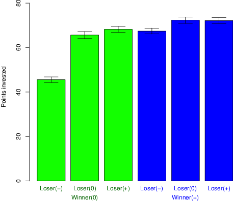
As seen in Figure 1, average investments varied considerably across conditions. We conducted a linear regression, with the condition – winner’s impact and loser’s impact – their interaction, and experiment round as predictors; variance was clustered by subject to control for the multiple decisions made by each subject.⁷ Most interesting from a social perspective is that investments were higher when the loser’s impact on the winner’s prize was positive and vice versa (t(108)=3.10, p=.002). In addition, when the winner had a positive impact on the prize, investments were higher (t(108)=2.73, p=.007). While this may seem intuitive, it is important to remember that even when winning in Winner(+), one still loses three-quarters of a point for every point invested. The interaction between Winner and Loser impacts was also significant, and seems to arise mostly from the low investment in the Winner(0)*Loser(-) condition (t(108)=-2.03, p=.045).

---

Figure 1: Average investments for the six conditions pertaining to the winner and the loser’s impacts on the winner’s prize. Error bars represent standard error of the mean.

---

---

Figure 2: Average prizes (darker bars) and investment—prize gaps (lighter bars) for the six conditions pertaining to the winner and loser’s impacts on the prize. Numbers above bars present the size of the investment-prize gap.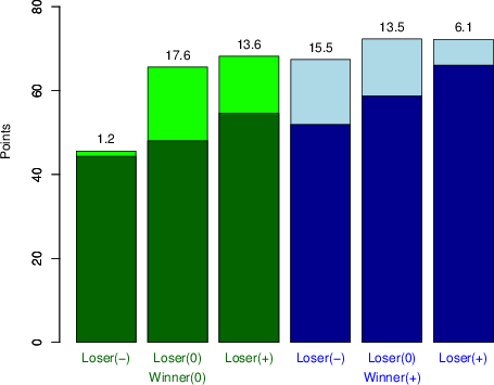

---

There was a significant effect of round, in that investments increased over rounds (t(108)=7.28, p<.001). However, after the first five rounds, investments reached a plateau; analyzing rounds 6-16, we observed no further effect of round (t(108)=1.20, p=.234). All of the other abovementioned effects remained the same.

2.6  Earnings (Q3)

Across all conditions, the average investment was 65.4 points, well over the average of the prize won, at 54.2 points. That is, subjects exhibited significant overinvestment, in that they invested (together) more than the prize they gained. We compared investments in each of the six conditions to their average prize: The average prizes and the investment—prize gaps in the six conditions are presented in Figure 2. As shown, investments were higher than the prizes in all conditions except in the Winner(0)*Loser(-) condition, and the difference was marginal in the Winner(+)*Loser(+) condition (t_{Winner(0),Loser(-)}(17)=0.42, p=.681; t_{Winner(0),Loser(0)}(15)=3.69, p=.002; t_{Winner(0),Loser(+)}(19)=3.81, p=.001; t_{Winner(+),Loser(-)}(17)=7.78, p<.001; t_{Winner(+),Loser(0)} (15)=5.98, p<.001; t_{Winner(+),Loser(+)}(19)=1.99, p=.061). This means that compared to not competing at all – and keeping their initial endowment – subjects in most conditions lost money from competing.

We submitted the investment-prize gap variable to a linear regression, with the winner’s impact and the loser’s impact, their interaction and round as predictors, and with the variance clustered by subject (See Table A3 in Appendix II for the regression results). There was a significant interaction between the Winner and Loser impacts (t(108)=-3.64, p<.001). As can be seen in Figure 2, this is mostly due to the smaller gap between investments and prizes in both the Winner(+)*Loser(+) and the Winner(0)*Loser(-) conditions. We return to this finding in the Discussion.

There was a significant effect of round, in that the gap increased (i.e., earnings decreased) over rounds (t(108)=7.21, p<.001). However, this effect was due to the first five rounds (as above); when analyzing rounds 6-16, there was no effect of round (t(108)=-0.77, p=.444), and all other effects remained the same.

---

Figure 3: Changes in investments between consecutive rounds, following win and loss, and linear predictions lines – averaged over winner and loser impact conditions. Circle sizes indicate the relative number of observations.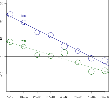

---

2.7  Investment dynamics (Q4)

As mentioned above, we observed a slight increase of investments over rounds, but this increase was limited to the first five rounds. That is, after a short period, which could perhaps indicate practice in the game, investments remained similar and did not escalate over time.

Our setting of repeated decisions enabled us to examine whether contestants react differently to winning (versus losing) when deciding on their subsequent investment. We tested whether there is an influence of the outcome in the previous round – winning or losing, and the actual prize won – and whether there are different dynamics in the different conditions (Winner and Loser impacts). We calculated the difference in investments between consecutive rounds, and submitted this variable to a linear regression model (again with variance clustered by subject). The outcome (win or loss),⁸ the size of the prize won, one’s previous investment, the conditions – winner’s and loser’s impacts – their interaction, and experiment round were the predicting variables.

As can be seen in Figure 3, there was a significant impact of winning versus losing: After winning, the subsequent investment was smaller, by an average of 5.4 points; after losing, investments increased, by an average of 14.4 points (t(108)=-3.46, p=.001). The previous investment had a significant effect, probably reflecting regression to the mean (t(108)=-5.87, p<.001). There was also a significant interaction between the outcome and previous investment (t(108)=2.46, p=.016).

In addition, the differences between consecutive investments were larger in the Winner(+) condition than in the Winner(0) condition (t(108)=2.39, p=.018); differences were larger the more positive the impact the loser had on the winner’s prize (t(108)=2.69, p=.008). There was also a significant interaction between the loser’s and the winner’s impacts (t(108)=-2.05, p=.043). The effect of the loser’s impact on the prize was moderated by the winner’s impact on their own prize: When it was positive, the loser’s impact had less of an effect. There were no significant interactions of the winner or loser’s impact conditions with the outcome (win or loss; all p’s >.41). Differences only slightly increased over rounds (t(108)=1.89, p=.062). See Table A4 in Appendix II for the regression results.

3  Discussion

This study examined investment behavior in competitions in which the contestants’ investments may affect their prize. As in many competitive situations in the world, and like previous studies (Cohen & Shavit, 2012; Coughlan & Plott, 1997; Dechenaux & Mancini, 2008; Hart et al., 2015; submitted; see review in Dechenaux et al., 2015), subjects in the experiment invested heavily, arguably too much, in the competition.

Importantly, investments differed according to how they might have affected the competition prize. Investments were higher when the loser’s investment increased the winner’s prize, and lower when the loser’s investment decreased the prize. We also observed higher investments when the winner’s investment increased the prize. Investments were high even though in some cases they led to lower overall earnings compared to competitions in which the prize did not depend on investments. The pattern of investments in the different competitions suggests that the subjects considered the overall pie, in that they were more motivated when their investments increased the aggregate revenue, and did not seek to hurt their opponents.

Investments exceeded the prize amounts in almost all conditions. Yet, there was a smaller gap between the investments and the prize in two of the conditions: When the winner and the loser both had a positive impact on the prize (Winner(+)*Loser(+) condition), and when the loser’s investment diminished the winner’s prize (Winner(0)*Loser(-) condition). These two conditions had higher earnings and less waste than in the other conditions. Notably, the smaller gaps between investments and prizes in the two conditions arose from different reasons. In the Winner(0)*Loser(-) condition, subjects invested much less than in the other conditions, and so the prize did not much decrease; thus the invested amounts were more similar to the prize. Conversely, in the Winner(+)*Loser(+) condition, subjects’ investments were high but the prize itself increased by a quarter of the summed investments; that is, a significant part of the investments was “returned” via the increase of the prize, leading to a smaller gap between the investment and the prize compared to other conditions.

As for investment dynamics, corroborating previous findings (Engelbrecht-Wiggans & Katok, 2007; Hart et al., 2015; submitted), subjects changed their investments between consecutive rounds in light of their previous outcome (win or loss): After winning, investments decreased; after losing, investments increased. This pattern was observed in all conditions, demonstrating that merely winning (or losing) plays a larger role in determining subsequent investments than does the amount of the prize. Moreover, these reactions remained throughout the rounds of the experiment, suggesting that subjects did not move toward a “correct” response over time through adjusting their investments in light of having invested too much or too little, but in fact responded to their outcome in the previous competition.

In sum, high investments in competition can be considered wasteful and undesirable when the contestants’ investments do not change the social welfare or their own welfare – in cases of political lobbying or rent-seeking activities. They may also be undesirable when contestants’ activities decrease the pie – for example by spending resources which could be used for other purposes, or by harming one another physically or financially (as in wrestling and lawsuits, respectively). Therefore, better understanding of investment behavior can help in designing the proper incentives via dependencies of the prize on investments so as to achieve the desired behavior. In order to discourage investments in these cases, one can plan the benefit structure so that contestants incur higher costs – via diminishing the prize – the higher (or longer) the competition. In contrast, when contestants’ investments increase social welfare (such as additional knowledge, innovative products or beautiful paintings), high investments could be construed as desirable. In order to encourage investments in such cases, prizes could be set so that they increase with the contestants’ aggregate effort.

4  References

---

Table A1: Equilibrium strategies, predicted investments and gains.

Winner Impact	Loser Impact	Equilibrium Strategy	Pred. Max. Invest	Pred. Mean	Pred. Gain
Winner(0)	Loser(-)	F(x)=4*(-1)*ln(1-0.25*x/96)	~85	40.7	0
	Loser(0)	F(x)=x/96	96	48	0
	Loser(+)	F(x)=4*ln((96+0.25*x)/96)	~109	56.8	0
Winner(+)	Loser(-)	F(x)=4*(1-exp(-0.25*x/96))	~110.5	57.9	0
	Loser(0)	F(x)=4*(1-96/(96+0.25*x))	128	70.1	0
	Loser(+)	F(x)=4*(1-(96/(96+0.5*x))^0.5)	149.3	85.3	0

---

Appendix I: Theoretic Predictions

We denote the two contestants by A and B, each choosing their strategy of investment, which is a distribution of a nonnegative random variable (X and Y, respectively). In any given game, contestant A’s investment will be x from distribution X, and contestant B’s investment will be y from distribution Y. We define a,b ≥ 0 to be the contestants’ respective mean investments in the contest game. Each contestant can invest only up to a certain amount of resources (their respective endowments), denoted by {r_A, r_B}. Each contestant also has a certain valuation for the prize, denoted by {v_A, v_B}.⁹ The resource endowments and valuations are public information.

In our setting, the contestant who invested more wins the prize; if the two contestants tie, each gets half of the prize. All contestants, regardless of winning or losing, always pay their investment. This means that the payoff function for contestant A (the payoff function for contestant B is the same, substituting y for x and v_B for v_A) is as follows.

The value of v_A=v_B=96, and both contestants’ endowments are equal to 96 (r_A=r_B=96). β denotes (1-winner’s impact), and δ denotes the loser’s impact on the winner’s prize. In our setting, the value of β is either 1 or 0.75 (Winner(0) and Winner(+), respectively). The value of δ is either 0.25, 0, or −0.25, in the Loser(-), Loser(0) and Loser(+) conditions, respectively.

The best response to each investment of the opposing contestant is, of course, to invest just slightly above. This response leads to winning at the lowest cost. Best-responding in such a manner, however, leads to an escalation which could get to a maximum investment, at which point the best-response would be to invest nothing – which, in turn, would start the cycle again. The theoretic solution for various parameter values is therefore in mixed strategies.

Let us start with the simple case in which the prize value is fixed at 96 points (v_A=v_B =96,  β =1,  δ =0). In this case, as aforementioned, each investment y is a best response to an investment of (y−1) points. Thus, one should give an equal weight to each of the possible options in the range of zero to 96 points. The equilibrium strategies are therefore: X=Y=U[0,96], and the mean investments are: a=b=48.

Baye et al. (2012) present the game theoretic model and equilibria of a contest similar to that used in our experiment, which allows for various dependencies (termed “spillovers”) of the prize on the contestants’ investments (i.e., different values of β and δ ). However, an important difference between the experimental conditions and Baye et al. is that in our setting, subjects could not invest more than 96 points in any condition (that is, as aforesaid, r_A=r_B=96). Adapting the Baye et al. model to our setting and using our parameters, subjects in some conditions are predicted to invest much more than 96. Table A1 presents the theoretical predictions – equilibrium strategies, predicted investments and gains – for all six conditions without capping the investments at 96.

Only in two conditions (the first two lines in Table A1) the predicted investment remains in the range of zero to 96 points: Winner(0)*Loser(-) and Winner(0)*Loser(0). In the other conditions, the maximum predicted investment exceeds 96. Hence, the Baye et al. (2012) model cannot be used to make predictions for these settings.

Nevertheless, the predicted ordinal relation between investments fits the observed values in all six conditions: The lowest investment by far is in the Winner(0)*Loser(-) condition, followed by Winner(0)*Loser(0), Winner(+)*Loser(-) and Winner(+)*Loser(0); investments in the Winner(+)*Loser(0) and Winner(+)*Loser(+) are the highest among our settings. That is, in line with the theoretic predictions, positive impacts increased the investments, whereas negative impacts led to lower investments. Further, and again in line with the predictions, the loser’s impact had a smaller effect on investments compared to the winner’s impact.

Appendix II: Regression Results

See Tables A2–A4.

Appendix III: Experiment Instructions¹⁰

---

Table A2: Linear regression model predicting investment.

	Coefficient	S.E.	t	p-value
Wself	43.023	15.765	2.73	0.007
Wopp	27.035	8.722	3.10	0.002
Wself*Wopp	-141.668	69.777	-2.03	0.045
round	1.754	0.241	7.28	0.000
_cons	50.342	2.855	17.63	0.000
N=1728; S.E. adjusted for 108 clusters. F(4,107)=21.63, p<.001; Model R2=0.122, RMSE=31.750

---

---

Table A3: Linear regression model predicting the investment—prize gap.

	Coefficient	S.E.	t	p-value
Wself	3.149	10.600	0.30	0.767
Wopp	2.593	5.903	0.46	0.661
Wself*Wopp	-172.042	47.223	-3.64	0.000
round	1.638	0.227	7.21	0.000
_cons	-2.862	2.265	-1.26	0.209
N=1728; S.E. adjusted for 108 clusters. F(4,107)=17.10, p<.001; Model R2=0.044, RMSE=41.353.

---

---

Table A4: Linear regression model predicting changes between consecutive rounds.

	Coefficient	S.E.	t	p-value
Previous	-0.384	0.065	-5.87	0.000
win	-2.821	0.814	-3.46	0.001
Prev*win	0.100	0.041	2.46	0.016
Wself	18.360	7.670	2.39	0.018
Wopp	12.200	4.527	2.69	0.008
Wself*Wopp	-69.711	34.022	-2.05	0.043
Wself*win	5.074	10.166	0.50	0.619
Wopp*win	2.847	6.577	0.43	0.666
Wself*Wopp*win	40.785	49.745	0.82	0.414
round	0.318	0.169	1.89	0.062
_cons	0.634	1.442	0.44	0.661
N=1356; S.E. adjusted for 108 clusters. F(10,107)=11.95, p<.001; Model R2=0.265, RMSE=25.098.

---

You will now participate in a game in which each of two players decides how much to invest in a contest, in multiple rounds. In each round, the contest winner gets a prize.

The amount you will receive at the end of the experiment is determined by your decisions and those of the other participants.

Please read the instructions carefully.

After reading the instructions, and during the entire experiment – if you have any questions, please raise your hand and one of the experimenters will approach you. Please keep quiet during the entire experiment.

The game will go as follows:

The game includes 16 rounds.

In each round, each of you has a box and a fixed number of points.

Each player will have 96 points in each round.

You may invest in the box any number between 0 and 96. The number you type will constitute your investment. Uninvested points will remain yours.

The player who invested more in the box, will win that round’s contest and wins the prize.

If the two players invested the same amount – each will receive half of the prize.

The size of the prize you will get if you win depends on your investment and the other player’s investment as follows:

The initial size of the prize is 96 points.

Winner(+):

Each point you invest will add 0.25 points (a quarter of a point) to the prize.]

Loser(+) / Loser(-):

Each point the other player invests will add / subtract 0.25 points (a quarter of a point) to the prize.]

Note that investment are non-refundable – whether you win or lose the contest.

Therefore, in a round in which you did not win, your total will be 96 minus your investment.

In a round in which you won, your total will be 96 minus your investment plus the prize as described above.

In each round the computer will randomly select your opponent from the participating players.

Your characteristics and those of the opposing player will appear on each screen in which you have to make a decision.

And the payment?

The computer will calculate the number of points you have left and add the prize – if you received it – in this round.

At the end of every round you will see the round summary: Your determining investment, the determining investment of the other player, and whether you got a prize – and so, your corresponding total for this round.

At the end of the game, the computer will sum up the totals for all rounds, and points will be exchanged for shekels according to the following exchange rate: Every 70 points equals one shekel.

*

Philosophy, Politics and Economics (PPE) Program, University of Pennsylvania. Email: einavi@gmail.com.

#

The Federmann Center for the Study of Rationality, and School of Education, The Hebrew University of Jerusalem.

The work reported in this paper was supported by Israel Science Foundation Grant 121/11 to Yaakov Kareev.

Copyright: © 2016. The authors license this article under the terms of the Creative Commons Attribution 3.0 License.

1

For an exception, see Baik, Chowdhury and Ramalingam (2014). When both contestants’ resources are very scarce or very abundant, the intensity of conflict is diminished; in these cases, people prefer to keep their resources rather than compete.

2

The pie may be maximal when both contestants invest zero, or when one of them invests the minimum amount and the other invests zero – depending on the allocation rule when both contestants sit out the competition.

3

The case in which the winner’s investment decreases the prize is not very interesting in our setting: One decreases one’s expected earnings the more one invests in all situations, since investments are non-refundable.

4

The exact equilibrium strategies, predicted investments and earnings according to the Baye et al. (2012) framework, in which contestants’ investments are not capped, are presented in Appendix I.

5

Interestingly, Chowdhury and Sheremeta (2011) argue that even positive impacts can yield different investment patterns (and equilibria), depending on the contestants’ perceptions. For example, if one gives more weight to the fact that if one loses one would have a higher cost than the winner, one would invest less; in contrast, if one paid more attention to the lower cost (or higher prize) if one wins, one would invest more.

6

The reader may note that, in the Loser(-) and the Loser(+) conditions, the winner could derive the loser’s investment from the prize they themselves received. However, pilot experiments (n=96) that were compared to our published data (Hart et al., 2015; n=96) showed no difference in investments between conditions in which subjects were explicitly told the opponent’s exact investment, and conditions in which they were told only whether they invested more or less than their opponent. With these two extremes having no effect on behavior there is no reason to suspect that the mere possibility of the winner to laboriously calculate the opponent’s investment could have made a difference in the current study.

7

This method of clustering the model variance by subject corrects for each subject’s repeated observations across time; see e.g., Petersen (2009) and Williams (2000). These analyses were conducted using STATA’s variance cluster option in linear and logistic regression (StataCorp. 2009). See Table A2 in Appendix II for the regression results.

8

The analysis did not include ties, since it is not clear whether subjects treat these situations as wins or losses, and this may differ between subjects.

9

This notation follows that of S. Hart (2014). Similar notations are used by Baye et al. (1996), Hillman and Riley (1989), and Che and Gale (1998).

10

N is smaller in this regression than in those above for two reasons: 1) we did not include the 132 instances of ties (N=264); 2) the last round (round 16) could not be included in this analysis since there can be no subsequent change in investment after the last round.

This document was translated from L^AT_EX by H^EV^EA.