Judgment and Decision Making, Vol. 11, No. 2, March 2016, pp. 185-196

Prospect Theory predicts that people tend to be more risk seeking if their reference point is perceived as a loss and more risk averse when the reference point is perceived as a gain. In line with this prediction, Franken, Georgieva, Muris and Dijksterhuis (2006) showed that young adults who had a prior experience of monetary gains make more safe choices on subsequent decisions than subjects who had an early experience of losses. There are no experimental studies on how experiencing prior gains and losses differently influences young and older adults on a subsequent decision-making task (the Iowa Gambling Task). Hence, in the current paper, adapting the methodology employed by Franken et al.’s (2006), we intended to test the generality of their effect across the life span. Overall, we found that subjects who experienced prior monetary gains or prior monetary losses did not display significant differences in safe/risky choices on subsequent performance in the Iowa Gambling task. Furthermore, the impact of prior gains and losses on risky/safe card selection did not significantly differ between young and older adults. These results showed that the effect found in the Franken et al.’s study (2006) is limited in its generality.

Keywords: decision making, Iowa Gambling Task, risk taking, aging, older adults.

1  Introduction

A large body of research has demonstrated that the presentation of choices in terms of gains and losses influences how people make decisions (Tversky & Kahneman, 1981). Indeed, according to Prospect Theory, people tend to be risk averse in the domain of gains and risk seeking in the domain of losses (Kahneman & Tversky, 1979). This effect holds up well in experiments where subjects are asked to make forced choices between two hypothetical options in either the gain or loss domain (for example see Mayhorn, Fisk & Whittle, 2002; Kim, Goldstein, Hasher & Zacks, 2005; Tversky & Kahneman, 1981). However, in a more realistic scenario where an individual has just lost €3000 in an investment in shares that have gone sour, how would this loss experience affect a subsequent investment decision? Will people tend to risk more or less than they would in a scenario where they have just experienced a gain? Little research has examined the effect of prior gains and prior losses on subsequent decisions involving the potential of either monetary gains or losses. There are notable exceptions. For instance, Thaler and Johnson (1990) investigated, in a series of experiments, the impact of prior gains and losses on risky choices and found, contrary to Prospect Theory, increased risk seeking following prior gains. However, the scenarios used by Thaler and Johnson (1990) were rather abstract, as they consisted of forced choices between options with clearly defined outcome probabilities. This situation is, therefore, rather different from the investment scenario previously described where no outcomes with clear probabilities of occurrence can be identified. If anything, while investment decisions are known to carry some risk, it is difficult, if not impossible, to quantify this risk due to the relatively unpredictable behavior of share prices.

In order to assess the impact of prior gains and losses on a subsequent monetary decision-making task, Franken, Georgieva, Muris and Dijksterhuis (2006) employed the Iowa Gambling Task (IGT; Bechara, Tranel & Damasio, 2000), a laboratory task typically used to more closely mimic those uncertain scenarios associated to financial decisions occurring in real life. In this task, people usually select 100 cards from four decks with the aim to maximise their monetary gain at the end of the game. When subjects select a card, they always receive money. However, for some cards, subjects also incur a monetary penalty. The four decks from which cards can be selected have different characteristics that are unknown to the subjects. When selecting from Decks C and D, the amount of money received is small, thus, given the relatively small size of the monetary penalties, persevering in selecting cards from these two decks will assure monetary gains in the long term. On the contrary, when selecting from the other decks (A and B) a larger amount of money is received, however the size of the occasional monetary penalties are sufficiently large to assure monetary losses in the long term. Hence, selections of cards from Decks C and D can be considered safe and advantageous, while selections from Decks A and B can be considered risky and disadvantageous. Subjects should discover these characteristics of the decks while playing the IGT (Bechara, Damasio, Tranel & Damasio, 2005).

In Franken et al.’s study (2006), a sample of young adults firstly performed a manipulated version of the IGT where subjects ended up either gaining or losing, irrespectively of the strategy used, a fixed amount of money. This provided the basis for either the prior gain or loss conditions of their study. Subsequently, subjects performed the standard version of the IGT (Bechara et al., 2000) with the initial endowment being the amount of money either gained or lost in the previous manipulated task. This amount was positive for subjects in the gain condition and negative for subjects in the loss condition. Franken and colleagues (2006) claimed to show that young adults who had an early experience of gains made more advantageous/safe choices in the IGT than subjects who had an early experience of losses, thus supporting Prospect Theory. However, they also found that the significant differences between the gain and the loss groups were confined to Blocks 2 and 3 out of a total of five blocks in the IGT, each comprising twenty selected cards.

The methodology employed by Franken and colleagues (2006) could be used to assess the impact of experiencing monetary gains or losses on subsequent risk seeking or risk averse behavior across the life span. According to Prospect Theory, we should expect risk aversion in the gain domain and risk seeking in the loss domain also among older adults. However, given the lack of empirical data on this issue, it is unclear whether this prediction is correct. Interestingly, the literature about the effect of framing on decision making across the life span has provided a mixed pattern of results on age-related difference in risk averse and risk seeking behavior that are not always consistent with Prospect Theory (Best & Charness, 2015). Indeed, in some studies older adults were found to be more risk averse in the loss domain than younger adults (Mikels & Reed, 2009; Nielsen, Knutson & Carstensen, 2008; Samanez-Larkin et al., 2007; Thomas & Millar, 2012). For instance, in a task where subjects could select from either a sure gain (or a sure loss) or a risky gamble, Mikels and Reed (2009) reported that both young and old adults tended to avoid the risky gamble in the gain frame (i.e., when the gambling information was presented positively in terms of gains). However, in the loss frame (i.e., when the gambling information was presented negatively in terms of losses), older adults were more risk averse than younger adults. Conversely, other studies claimed to show that older adults were more risk averse than younger adults in the gain domain (Albert & Duffy, 2012; Lauriola & Levin, 2001; Weller, Levin & Denburg, 2011), and that older adults were more risk seeking in the loss domain than younger counterparts (Lauriola & Levin, 2001; Mather et al., 2012). Finally, other studies did not detect significant age-related selection differences as a function of either gain or loss domains (Samanez-Larkin et al., 2007; Thomas & Millar, 2012). In summary, on the basis of these studies, it is currently unclear whether there is an age-related effect on decision making in gain vs. loss domains. Moreover, as mentioned above, none of the aforementioned age-related studies was designed to investigate the impact of prior gains and losses on subsequent decisions. Therefore, exploring how experiencing prior gains and losses differently influences young and older adults decision-making processes may be particularly informative on the analysis of taking risky decisions in the domain of gains and losses across the life span.

The purpose of the current study was to test the generality of the effect reported in Franken and colleagues’ study (2006) in a sample of young and older adults. In particular, adapting the methodology employed by Franken et al. (2006), we intended to assess whether prior gains and losses differently affect young and older adults’ proneness to take safe/risky choices in a subsequent task. If older adults are less risk seeking in the loss domain than younger adults (e.g., Mikels & Reed, 2009; Nielsen et al., 2008; Samanez-Larkin et al., 2007; Thomas & Millar, 2012), we would expect that in the standard IGT, particularly so following prior losses in the manipulated IGT, elderly would select less disadvantageous cards (i.e., from Decks A and B) than young adults. Conversely, if older adults are more risk seeking in the loss domain (Lauriola & Levin, 2001; Mather et al., 2012) than younger adults, then, following prior losses in the manipulated IGT, they should select more disadvantageous cards (i.e., from Decks A and B) in the standard IGT. If, on the other hand, young and old adults are equally sensitive to the impact of prior losses, as in Franken and colleagues’ study on young adults (2006), we should find comparable profiles in the loss and gain conditions for both young and old adults. Finally, given Franken et al.’s findings (2006), it is expected that any difference between prior gains and prior losses conditions should more likely emerge in the second and third blocks of the game.

In the present study we also included the Positive and Negative Affect Schedule (PANAS; Watson, Clark & Tellegen, 1988) and the Rosenberg Self-Esteem Scale (RSE; Rosenberg, 1979) in order to assess whether (a) the experimental manipulation intended to induce gains and losses may impact on affect states and self-esteem and (b) the extent to which any change in affect state and self-esteem could be associated to more or less safer/riskier behaviours.

2  Method

---

Table 1: Descriptive statistics of young and older adults as a function of experimental conditions (Prior Gain vs. Prior Loss).

	Young adults					Older adults
	Prior Gain		Prior Loss			Prior Gain		Prior Loss
	(n = 25)		(n = 25)			(n =34)		(n = 38)
Subject characteristics	M	SD	M	SD		M	SD	M	SD
Age	24.44	3.66	24.12	4.19		68.15	6.02	67.92	6.68
Years of education	15.32	2.10	14.68	2.19		14.62	4.25	14.55	3.67
Vocabulary	42.36	4.21	42.92	4.54		45.15	3.43	46.21	5.01
MMSE						28.74	1.40	28.61	1.57
Note: Maximum vocabulary score = 50;Maximum MMSE score = 30

---

2.1  Subjects

Fifty young adults (M_age = 24.28; SD = 3.90; age range: 19–33; 39 females) and 72 older adults (M_age = 68.03; SD = 6.33; age range: 60–86; 43 females) participated in this experiment. Older adults were recruited through the local branch of the University of Third Age located in northern Italy, where they attended several cultural activities (i.e., lessons, conferences, etc.). Younger adults were undergraduate students and received course credits for participating.

About half of the subjects in each age group were randomly allocated to either the prior gain (n = 59; 25 young adults; 34 older adults) or to the prior loss condition (n = 63; 25 young adults; 38 older adults). Subjects filled out a general demographic questionnaire so that we could exclude subjects with a history of psychiatric or neurological disorders and substance abuse. In addition, only for older adults, an initial screening was made using the Mini Mental State Examination (MMSE; Folstein, Folstein & McHugh, 1975) in order to exclude subjects with a score lower than 26. No subjects was excluded on the basis of above criteria. A vocabulary test (extracted from the Primary Mental Ability; Thurstone & Thurstone, 1963) was also presented to subjects in the study to assess crystallized intelligence. All subjects completed and accepted an informed consent form prior to the beginning of the experiment. Descriptive statistics on age, years of education, MMSE, vocabulary scores are reported in Table 1.

Results of two 2 (Age: Young vs. Old) by 2 (Experimental Conditions: Prior Gain vs. Prior Loss) analyses of variance (ANOVA) conducted on years of education and on performance in the vocabulary test showed that older subjects outperformed younger subjects in vocabulary scores, F(1, 118) = 14.17, MSE = 19.20, p < .001, η_p² = .11. No significant differences in years of education was detected between age groups, F(1, 118) = .45, MSE = 11.14, p =.501, η_p²= .004. Years of education and vocabulary did not differ between prior gain and prior loss conditions (Fs ≤ 1.01, ps ≥ .317) and the interactions between age and experimental conditions were not significant (Fs ≤ .219, ps ≥ .641).

2.2  Materials

---

Table 2: Prototypical pattern of gain-loss of every 10 picks from each of the four decks both in the original IGT and in the manipulated IGT loss and gain versions.

	Original IGT				Manipulated IGT
Deck card sequence	A	B	C	D	ABCD loss version	ABCD gain version
1	100	100	50	50	50	150
2	100	100	50	50	50	150
3	100, –150	100	50, –50	50	50, –200	150, –200
4	100	100	50	50	50	150
5	100, –300	100	50, –50	50	50, –200	150, –200
6	100	100	50	50	50	150
7	100, –200	100	50, –50	50	50, –200	150, –200
8	100	100	50	50	50	150
9	100, –250	100,–1250	50, –50	50	50, –200	150, –200
10	100, –350	100	50, –50	50, –250	50, –200	150, –200

---

2.2.1  Experimental Tasks

The experimental tasks were adapted from Franken and colleagues’ study (2006). They consisted in a Manipulated IGT (M-IGT) and in the Original IGT (O-IGT; Bechara et al., 2000). The M-IGT was a modified and shorter computer-based version of the O-IGT. It consisted of 40 trials in which four decks of cards (A, B, C, D) were presented on a computer screen. Subjects were required to select one card at the time and they were told that their aim was to try to win as much money as possible. They started the game with no endowment (i.e., €0). Furthermore, subjects were told neither the number of trials (i.e., 40) nor the schedule of reinforcements; however, they were told that each card would always carry a reward as well as, in some cases, a penalty. There were two versions of the M-IGT: a winning version and a losing versions where, irrespective of the strategy used to select the cards, a final gain or a loss, respectively, was obtained. The winning and losing versions of the M-IGT had predetermined and symmetrical patterns of gains and losses (the proportion of cards with net losses and net gains was 50% in each deck). In the losing version of the M-IGT, turning any card from Deck A, B, C or D provided an immediate return of €50, while, in each deck, in five picks every ten cards, a penalty of €200 occurred. In the winning versions of the M-IGT, the reward for any card was €150, while, in each deck, in five picks (every ten cards) a penalty of €200 occurred (see Table 2 for prototypical patterns of schedules of rewards and punishments used in the M-IGT). Therefore, subjects ended with either about a €2000 win or with about a €2000 loss, irrespectively of the strategy used. The winning and the losing versions of the M-IGT were used in the prior gain and prior loss conditions, respectively.

In the standard O-IGT, as for the M-IGT, subjects had to select cards from four decks (A, B, C, D) displayed on a computer screen. Each deck was associated with more or less favorable contingencies of wins and losses of money (the contingencies used were the same proposed in the study of Bechara et al., 2000). Thus, as shown in Table 2, selecting from decks A and B leads to losses in the long term, while selecting from decks C and D leads to gains in the long term. Subjects were simply told that some decks were advantageous, while others were disadvantageous and that their aim was to gain as much as possible by the end of the game. However, importantly, subjects did not know either the total number of cards to be selected nor which were the advantageous and the disadvantageous decks. When a card was selected from the two advantageous decks (i.e., C and D) an immediate win of €50 was always delivered, while from the two disadvantageous decks (i.e., A and B) an immediate win of €100 was always delivered. However, as well as sure wins, occasional losses also occurred when cards were selected (as shown in Table 2). In particular, if subjects constantly selected from Decks A and B, after every ten selections, each deck provided a cumulative loss of €250. Conversely, if subjects constantly selected from Decks C and D, after every ten selections, each deck leads to a cumulative gain of €250, so these decks are advantageous in the long run.

Performance in the O-IGT was scored in two way: (a) as the number of cards selected from advantageous decks minus the number of cards selected from disadvantageous decks for each block of twenty cards (1–20, 21–40, 41–60, 61–80, 81–100) and (b) as the mean frequency of cards selected form Decks A, B, C, D over the task. The first measure represents the standard analysis used to assess performance in the IGT; the second measure provided the basis for a finer grained analysis of the type of decks selected over the course of the game. These two measures of the O-IGT were used as dependent variables in the subsequent analyses.

2.2.2  PANAS and Self-Esteem Scale

The Positive and Negative Affect Schedule (PANAS; Italian version Terraciano, McCrae & Costa, 2003; Watson, Clark & Tellegen, 1988) is a self-report questionnaire consisting of 10 items (adjectives) for the Positive Affect scale (PA) and 10 items for the Negative Affect scale (NA). For each adjective associated to an affect state, subjects are asked to rate, on a 5-point scale ranging from 1 (very slightly or not all) to 5 (extremely), the extent to which they experience each mood state “at the present moment”. The score of single items was summed, therefore possible total scores for both positive and negative affect scale could range from 1 to 50. Higher scores indicate higher levels of either positive or negative affect states.

The Rosenberg Self-Esteem Scale (RSES; Italian version Prezza, Trombaccia & Armento, 1997; Rosenberg, 1979) is a self-report questionnaire consisting of 10-item describing a series of statement measuring self-worth. Subjects have to respond to each item using a 4-point scale anchored at 1 (strongly disagree) and 4 (strongly agree). The scores obtained in the single items were added up, therefore possible total scores could range from 1 to 40. Higher scores indicate high levels of trait self-esteem.

2.3  Procedure

The order of tasks administration was the same for all subjects. Firstly, for screening purpose, subjects completed a demographic questionnaire, the vocabulary subtest drawn by Primary Mental Ability and, only subjects in the older age group, the Mini Mental State Examination. Subsequently, subjects carried out the Positive and Negative Affect Schedule (PANAS) and Rosenberg Self-Esteem Scale (RSES). After having completed the PANAS and RSES, subjects performed either the winning or the losing version of the M-IGT. In order to make the experience of gain and loss more salient, at the end of this task subjects who performed the winning M-IGT and subjects who performed the losing M-IGT were told that they either gained or lost more money than average on the task. Immediately after performing the M-IGT, subjects completed the PANAS and the RSES for a second time. Finally, they performed the O-IGT. Before starting the O-IGT, subjects were instructed that completely new rules applied to this game, as compared to the M-IGT, thus implying that they should use different strategies than those used in the M-IGT. Furthermore, they were informed that their prior gain or loss was the starting point for the second task. Hence, subjects in the prior loss and in the prior gain conditions started the O-IGT with an initial debt or credit of €2000, respectively. Subjects did not receive real money according to their final monetary win or loss.

2.4  Analysis

Firstly, to analyze how prior gains or prior losses affected risk taking behavior in general, and more specifically in young and older adults, a mixed analysis of variance (ANOVA) 2 (Experimental Conditions: Prior Gain vs. Prior Loss) by 2 (Age: Young vs. Old) by 5 (O-IGT Blocks: 1-to-5), was conducted on the number of advantageous (i.e., safe) minus disadvantageous (i.e., risky) selections in the O-IGT. Experimental Conditions and Age were between-subjects factors, while O-IGT Blocks was the within-subjects factor. Additionally, we performed follow-up independent-samples t-tests between prior gains and prior losses groups based on the a priori hypothesis that in Blocks 2 and 3 subjects in the prior gain group should select more advantageous choices than subjects in the prior loss group (Franken et al., 2006). This a priori follow-up was based on the finding of Franken and colleagues’ study (2006). In particular, on the basis of their data, the estimated average size of the effect of the gain vs. loss conditions on selecting more advantageous cards across Blocks 2 and 3 is d = 0.96. Hence, given our overall sample size, the power to detect this effect, for an alpha level of 0.05, was about 0.95.

Second, to analyze the strategy used in prior gains and prior losses experimental conditions, mean frequencies of decks’ selection in the O-IGT were analyzed using a four factors mixed ANOVA 4 (Deck: A, B, C, D) by 5 (O-IGT Blocks: 1-to-5) by 2 (Experimental Conditions: Prior Gain vs. Prior Loss) by 2 (Age: Young vs. Old). Experimental Conditions and Age were between-subjects factors and Deck and O-IGT Blocks were within-subjects factors. In this analysis we will primarily focus on any change in the decks’ selection over the course of the game and on any effect on decks’ selection of both Age and the Experimental Conditions.

Third, in order to assess whether the experimental manipulation influenced affect states and self-esteem, a three factors mixed ANOVA 2 (Experimental Conditions: Prior Gain vs. Prior Loss) by 2 (Time of measurement: Before M-IGT vs. After M-IGT) by 2 (Age: Young vs. Old adults) was conducted on scores from the PANAS and on Rosenberg Self-Esteem Scale. Since the results in the PANAS negative affect scale were severely limited by a floor effect (i.e., subjects selected a score of one most of the times), results concerning the negative affect state could not be meaningfully analyzed. Experimental Conditions and Age were between-subjects factors and Time of measurement was the within-subjects factors.

The significance level adopted for all analyses was 0.05, unless otherwise stated. Paired t-tests were used to follow-up significant F ratios. Since there were at most six pairwise comparisons, the significance level adopted for these follow-up analyses was 0.008.

3  Results

---

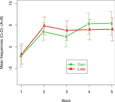
Figure 1: The mean difference between the frequency of advantageous (C+D) minus disadvantageous selections (A+B) for each of the five original IGT blocks 1-to-5 as a function of the prior gain and prior loss conditions. Bars indicate confidence interval. (See the appendix for tabular version.

---

3.1  Advantageous minus disadvantageous selections in the O-IGT

Blocks had a significant main effect, F(4, 472) = 15.03, MSE = 62.66, p < .001, η _p² = .113, indicating that subjects’ frequency of advantageous selections increased from Block 1 to Block 5. In particular, there were significant increments from Block 1 to Block 2, t(121) = 5.45, p < .001, Block 3, t(121) = 4.66, p < .001, Block 4, t(121) = 6.02, p < .001, and Block 5, t(121) = 5.61, p < .001. No significant differences occurred between Blocks 2 through 5, ts ≤ 1.73, ps ≥ .087. Overall, then subjects moved from selecting more from disadvantageous decks (A and B) to more advantageous decks (C and D). Figure 1 displays the mean difference between frequency of advantageous and disadvantageous selections of both starting conditions over the five blocks of the O-IGT. The main effect of age and experimental condition were not significant, Fs ≤ .06, ps ≥ .807. Neither was the two-way interaction between Blocks and Experimental Condition, F(4, 472) = .76, MSE = 62.66, p = .553, η _p² = .006. From the planned t-tests between gain and loss conditions at Blocks 2 and 3 no significant differences emerged: Block 2, t(120) = 0.90, p = .368; Block 3, t(120) = 0.87, p = .385. Overall, it appears that, contrary to Franken et al.’s study (2006), there was no significant differences in the impact of prior gains vs. losses on O-IGT scores. In particular, the planned t-tests failed to reject the null hypothesis of no difference between advantageous and disadvantageous selection at Block 2 and 3 despite this experiment had a power of 0.95 to detect an effect size of the magnitude obtained by Franken et al. (2006).

---

Figure 2: The mean difference between the frequency of advantageous (C+D) minus disadvantageous selections (A+B) for each of the five original IGT blocks 1-to-5 as a function of age group (young adults vs. old adults) for the prior gain and prior loss conditions. Bars indicate confidence interval.

---

The two-way Block by Age interaction was not significant, F(4, 472) = .75, MSE = 62.66, p = .557, η _p² = .006, indicating a similar performance in old and young adults over time. Similarly, the three-way interaction was not significant, F(4, 472) = .67, MSE = 62.66, p = .616, η _p² = .006. Figure 2 displays the mean difference between the frequencies of advantageous and disadvantageous selections as a function of the five blocks, the starting conditions and age groups. Overall, it appears that subjects started selecting more from advantageous decks relatively early in the game, however, unlike Franken et al. (2006), there was no significant difference between gains and losses conditions. Furthermore, the profile of the performance over time was comparable between age groups in both prior gains and prior losses conditions.

---

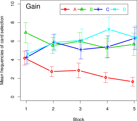
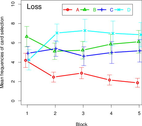
Figure 3: The mean frequencies of cards selected from each deck (A, B, C, D) by the five original IGT blocks 1-to-5 as a function of prior gain and prior loss conditions. Bars indicate confidence interval. (See the appendix for a tabular version.)

---

3.2  Mean frequencies of decks’ selection over the O-IGT

Deck (A, B, C, or D) had a significant main effect, F(3, 354) = 38.23, MSE = 41.20, p < .001, η _p² = .245. Planned comparisons indicated that subjects selected Deck A significantly less often than any other decks (ts ≥ 8.64, ps < .001). The two-way interaction Decks by Blocks was significant, F(12, 1416) = 7.57, MSE = 13.590, p < .001, η _p² = .06. Inspecting Figure 3, it can be noticed that over time subjects tended to select more readily from the advantageous Decks C and D and tended to avoid selecting the disadvantageous Deck A. However, it also appears that disadvantageous Deck B, i.e. the one delivering, on average, only one large loss every 10 selection, was selected frequently throughout the entire game. Finally none of the other interactions approached significance, Fs ≤ 1.01, ps ≥ .389. In summary, the analysis of frequencies of cards’ selections from the different decks showed that, irrespectively of the starting condition, subjects could rapidly identify Deck A as being disadvantageous and Decks C and D as being advantageous; however subjects found it difficult identifying, even at the latest stages of the game, the disadvantageous nature of Deck B. This most likely occurred because Deck B delivers large rewards frequently, but large losses rarely (1 out of every 10 cards) (for similar findings and considerations see Steingroever, Wetzels, Horstmann, Neumann & Wagenmakers, 2013).

3.3  PANAS positive affect scale and Self-Esteem Scale

The positive affect scale from PANAS showed a Time of measurement by Experimental Conditions interaction, F(1, 118) = 6.14, MSE = 8.84, p = .015, η _p² =.05. Indeed, positive affect decreased after performance on the losing version of the M-IGT (Before M-IGT: M = 31.13, SD = 4.95; After M-IGT: M = 29.86, SD = 6.20), t(62) = 2.21, p = .031, while it did not significantly differ in the winning version of the M-IGT (Before M-IGT: M = 29.83, SD = 5.68; After M-IGT: M = 30.17, SD = 6.34), t(58) = 0.66, p = .514. Moreover, the three-way interaction between Time of measurement, Experimental Condition and Age was significant, F(1, 118) = 5.64, MSE = 8.84, p < .019, η _p² =.05.

To better describe the three-way interaction, we conducted two separate follow-up analyses to assess the combined effect of experimental condition and time of measurement separately for the young and old age groups, respectively. In the younger adult group, a significant Time of measurement by Experimental Condition occurred, F(1, 48) = 10.04, MSE = 8.80, p = .003, η _p² = .17, indicating that positive affect decreased after performing the losing version (Before M-IGT: M = 32.84, SD = 5.88; After M-IGT: M = 30.88, SD = 6.25), t(24) = 2.18, p = .040, and increased after performing the winning version of the M-IGT (Before M-IGT: M = 28.88, SD = 5.71; After M-IGT: M = 30.68, SD = 6.13), t(24) = 2.33, p = .029. In the older adult group, no significant interaction occurred, F(1, 70) = .01, MSE = 8.87, p = .936, η _p² =.00, indicating that positive affect changed neither after performing the losing (Before M-IGT: M = 30.00, SD = 3.92; After M-IGT: M = 29.18, SD = 6.16), nor the winning version of the M-IGT (Before M-IGT: M = 30.53, SD = 5.64; After M-IGT: M = 29.79, SD = 6.56), ts ≤ 1.15, ps ≥ .259.

The Rosenberg Self-Esteem Scale showed a significant Time of measurement by Experimental Conditions interaction, F(1, 118) = 6.71, MSE = 2.31, p = .011, η _p² =.05, indicating a significant increase of self-esteem after the winning version of the M-IGT, (Before M-IGT: M = 31.04, DS = 3.93; After M-IGT: M = 31.64, DS = 4.39), t(58) = 2.10, p = .040, but not after the losing version of the M-IGT, (Before M-IGT: M = 31.31, DS = 4.13; After M-IGT: M = 30.87, DS = 4.66), t(62) = 1.64, p = .105. None of the other interactions approached significance, Fs ≤ 2.24, ps ≥ .137.

4  Discussion

The present study aimed to assess whether the experience of prior monetary gains and losses differently affect young and older adults’ subsequent choices in a decision-making task mimicking the uncertainty of real investment scenarios. To this aim, we adapted the methodology used by Franken et al. (2006). This also provided an opportunity to assess possible age effects. Young and old adults performed the classical version of the IGT after having performed a manipulated version of the IGT resulting in either a gain or a loss reference point.

Our results showed that, overall, subjects who experienced prior monetary gains or prior monetary losses did not display significant differences in safe/risky choices in subsequently performing the O-IGT. Furthermore, the impact of prior gains and losses on risky/safe choice behavior did not significantly differ between age groups. Our failure to detect an increased risk taking in the loss condition (or conversely greater risk aversion in the gain condition) on the subsequent selection of advantageous vs. disadvantageous decks is at odds with Franken et al.’s results (2006).

A lack of statistical power in our experiment is unlikely to account for our results. Given the absence of an age effect, we pooled both age groups in order to have an overall sample of 122 subjects against the 50 subjects of the Franken et al.’s study (2006). Hence, our overall sample included 2.5 times as many observations as the original sample size, thus providing a suitable size attempt to generalize previous findings (Simonsohn, 2015). Moreover, with a predicted effect size of d = 0.96, estimated from Franken et al.’s study (2006), our experiment had a probability of 0.95 to detect such an effect. Hence, it appears that, on the basis of the results of the present study, the effect reported in Franken and colleagues’ study (2006) is not a phenomenon that can be readily obtained in an experimental context that differs from the one originally adopted.

There are, indeed, methodological differences between the present study and the Franken et al.’s study (2006) that should be considered for the inconsistency in the results between the two studies.

Firstly, Franken and colleagues (2006) used real monetary remuneration as a function of task performance, while we did not. Hence, the absence of a monetary remuneration resulting from subjects’ winnings and losses on the O-IGT might have affected motivation in task performance (Mikels & Reed, 2009). Indeed, some studies showed that the type of reinforcement (real vs. no or fictitious money) could influence behavioral decision making (Hertwig & Ortmann, 2001; Weinberg, Riesel & Proudfit, 2014) and, in particular, risk aversion (Ferrey & Mishra, 2014; Holt & Laury, 2002). On the other hand, however, this type of evidence contrasts with other studies carried out using the IGT that failed to find significant differences in the rate of learning of IGT contingencies as a function of reinforcement type (e.g., Bowman & Turnbull, 2003; Fernie & Tunney, 2006). If real monetary reinforcement matters, we would expect subjects, at least in the gain condition, to learn faster in the Franken et al.’s study (2006) than in the present study.

In order to assess this hypothesis, we calculated the slopes measuring the learning rate in the IGT from the first to the third block of 20 trials in both the gain (i.e., 4.32) and the loss (i.e., 1.32) conditions of the Franken et al.’s study (2006) and we used these values as point estimates (i.e., as if these values were the mean of the null hypothesis to be used in a t-test).¹ The third block was used because at this point a slower performance was clearly detected in the loss condition over the gain condition in the Franken et al.’s study and because, following this block, performance in the gain and loss conditions tended to equate and reached asymptote. We then computed, for each of our subjects, these slopes for both gain and loss conditions and calculate their means and standard errors. For the gain condition the mean slope was 2.25 (SE = 0.815) and for the loss conditions the mean slope was 2.71 (SE = 0.705). We then performed one sample t-test against the point estimates obtained from Franken et al.’s study (2006). In the gain condition we obtained t(58) = –2.54, p = .018 against a point estimate of 4.32 (limits of the 95% CI: 0.618 and 3.881), while in the loss condition we obtained t(62) = 1.98, p = .058 against a point estimate of 1.32 (limits of the 95% CI: 1.305 and 4.123). These results indicate that slower learning rates emerged in the gain condition of our study as compared to Franken et al.’s study (2006). Moreover, the average learning rate in the first three blocks of the loss condition of our study was marginally faster than the average learning rate in Franken et al.’s study (2006). Overall, the comparison of the learning rates across the two studies seems to support the view that monetary rewards may have a positive impact on the learning rate in the gain condition, while in the loss condition these tended to be slower. For completeness, there were no significant differences in the slopes between the gain and loss conditions in our study, t(160) = 0.67.

Although the use of real vs. fictitious amounts of money may have contributed to the differences in the learning rates detected, it is important to consider that despite no real money being won/lost in our study, the experimental manipulation of gains and losses was effective in inducing changes in affect states. This suggests that subjects took the task seriously enough to be disappointed even when they lost fictitious amounts of money. Therefore, it seems premature to attribute the lack of an effect of the gain/loss manipulation on the learning rate in our study to the fact that no real money was used as incentive.

Secondly, the amount of fictitious money gained or lost in the M-IGT was different from that used in the Franken et al.’s study (2006). While Franken and colleagues (2006) used more realistic amount of money won or lost as a function of the modified IGT performance (i.e., a gain of €4 in the prior gain condition and a loss of €10 in the prior loss condition), in the present study subjects won or lost about €2000 as a consequence of their M-IGT performance. The high amounts of virtual money won or lost in the present study might have contributed further to the feeling that it was not a real task but just a game and it might consequently have influenced the strategy adopted by subjects during the subsequent O-IGT.

Furthermore, as a third difference, the amount of trials (i.e., 100 trials) presented in the modified IGT of Franken et al.’s study (2006) was longer than the amount of trials used in the present study (i.e., 40 trials). This difference might have affected early preferences for blocks in the subsequent O-IGT.

Despite these methodological differences between our and Franken et al.’s study (2006), it would be expected that, if the effect of prior gains/losses on the performance of the IGT is robust, it would be relatively easy to be obtained in a different experimental context.

The analysis we performed on decks’ selection helps to shed light on the strategy used by subjects and thus may help understanding why different outcomes were found in our and in Franken et al.’s study (2006). Overall, the mean frequencies of cards selected from each deck (A, B, C, D) across the five blocks of the IGT was comparable in prior gains and prior losses conditions. It is noticeable, and compatible with the learning of the contingencies of the IGT, that the frequency of choice of the disadvantageous Deck A decreased as the task progressed, and that the frequency of selection of the advantageous Decks C and D increased over the five blocks. Indeed, from Block 2 it is already evident that advantageous Decks C and D were selected more frequently than Deck A. However, and critically, the disadvantageous Deck B was selected with a similar frequency to Decks C and D across the entire game, irrespectively of the gains and losses conditions. Deck B features high frequency of relatively large gains and very infrequent large losses; thus, similarly to advantageous Decks C and D, it delivers infrequent net losses. A recent review by Steingroever and colleagues (2013) claimed to show that, across a very large set of studies using the IGT, it is common to observe large proportions of subjects promptly discarding the disadvantageous Deck A but persistently selecting the disadvantageous Deck B. This effect, called the “prominent Deck B” phenomenon, was reported in a variety of studies (e.g., Dunn, Dalgleish & Lawrence, 2006; Lin, Chiu, Lee & Hsieh, 2007; Toplak, Jain & Tannock, 2005). For instance, Lin and colleagues (2007) suggested that Deck B may be difficult to disregard due to its similarity to the advantageous Decks C and D; indeed, unlike Deck A, no or very few net losses are associated to all these three decks. This hypothesis is also supported by the results of a recent study where subjects were asked to try to lose, instead of winning, as much money as possible in the standard IGT (Wright, Rakow & Russo, 2015). Due to the reverse nature of the instructions, Deck B became a favorable deck; nonetheless, this tended to be selected as frequently as the now unfavorable Decks C and D.

On the basis of the above considerations and of the empirical evidence provided about the pervasive preference for the disadvantageous Deck B (Steingroever et al., 2013), it seems possible that a large proportions of the subjects in the loss group of Franken et al.’s study (2006) fortuitously showed a preference for Deck B very early in the IGT. This preference might have inflated the number of cards selected by subjects from disadvantageous decks: a selection pattern that persisted also in the early middle blocks of the game (we assume, on the basis of the evidence reviewed above, that Deck A would have been discarded relatively quickly). This hypothesis, however, could not be directly tested as no decks analysis is provided in Franken et al.’s study (2006).

The outcome of the present study provided further interesting results. Firstly, with respect to the issue of potential age related differences in performing the IGT, we found that both young and older adults learned to distinguish, in a comparable way, advantageous from disadvantageous decks relatively early in the game, and this learning was retained until the end of the task. Therefore, our findings add to the body of evidence showing age-related differences in performing the IGT are either minimal or non-existent (e.g., Henninger & Madden, 2010; MacPherson, Louise & Della Sala, 2002; Shneider & Parente, 2006).

Secondly we found, in line with Franken and colleagues’ study (2006), an increase of positive affect following monetary gains in the manipulated version of the IGT, and a decrement of positive affect following the monetary losses, albeit primarily in the young adults group; older adults did not report changes in positive affect. The absence of changes in positive affect among older adults seems to imply that elderly are less susceptible to the impact of monetary gains and losses than younger adults. However, and interestingly, previous studies reported that older adults displayed significantly lower levels of affect variability than young adults in association to both positive and negative daily events (e.g., Röcke, Li & Smith, 2009). Furthermore, studies on age-related differences in physiological reactivity on affective states (Levenson, Carstensen, Friesen & Ekman, 1991) reported a decline in physiological reactivity among older adults in emotional tasks. For instance, it has been reported that older adults show reduced physiological arousal when watching emotional movies (Tsai, Levanson & Carstensen, 2000) than younger adults. Hence, our results provide further empirical support to those studies reporting that older adults are less affectively reactive than younger adults to positive and negative stimuli (e.g., Röcke et al., 2009; Tsai et al., 2000). Finally, the absence of changes in positive affect following monetary gains and losses in older adults did not affect results on the manifestation of safe/risky behaviours in the IGT in the older group. Younger adults, despite showing changes in positive affect following the gain/loss manipulations, did not display differences in safe/risky choices as a function of prior gains and losses. Moreover, and interestingly, we found across subjects an increase of self-esteem following monetary gains in the manipulated version of the IGT. Hence, despite subjects showed changes in self-esteem following the winning version of the IGT, they did not display differences in safe/risky behaviors in the subsequent decision-making task.

In conclusion, although further work is required to gain a more complete understanding of the impact of prior gains/losses on decision making across the life span, our results showed that experiencing prior monetary gains and losses is unlikely to affect subsequent safe/risky decision behavior in both young and older adults. Hence, the results of the present study should serve as a warning that the effect of experiencing prior gains and losses on subsequent decision making is not easy to get. However, it is important to point out that this result was detected using a specific task aimed to mimic the uncertainty of real life investment scenarios. Therefore, future studies should try to extend the present methodology to different tasks to assess the generalizability of the present findings. Furthermore, we hope that this study provides the impetus for further research to be conducted on the impact of prior gains and losses on decision making across the life span.

References

Appendix: Means (M) and confidence intervals (95% C.I.) of Figures 1 and 3

---

Table A1: Confidence intervals and the mean difference between the frequency of advantageous (C+D) minus disadvantageous selections (A+B) for each of the five original IGT blocks 1-to-5 as a function of the prior gain and prior loss conditions. The values correspond to Figure 1 of the paper.

	Prior Gain		Prior Loss
	M	95% C.I.	M	95% C.I.
Block 1	–2.17	–4.58 – 0.24	–1.65	–3.98 – 0.68
Block 2	3.49	1.39 – 5.59	4.83	2.79 – 6.86
Block 3	2.34	–0.01 – 4.69	3.78	1.51 – 6.05
Block 4	5.32	2.89 – 7.76	3.97	1.61 – 6.32
Block 5	5.39	2.65 – 8.13	4.03	1.38 – 6.68

---

---

Table A2: Confidence Intervals and the mean frequencies of cards selected from each deck (A, B, C, D) by the five original IGT blocks 1-to-5 as a function of prior gain and prior loss conditions. The values correspond to Figure 3 of the paper.

	A		B		C		D
	M	95% C.I.	M	95% C.I.	M	95% C.I.	M	95% C.I.
Prior gain
Block 1	4.17	3.42 – 4.92	6.92	5.83 – 7.99	4.27	3.54 – 5.00	4.64	3.56 – 5.73
Block 2	2.73	2.19 – 3.27	5.53	4.65 – 6.40	5.88	5.05 – 6.71	5.86	4.92 – 6.81
Block 3	2.85	2.25 – 3.63	5.98	5.04 – 6.92	5.09	4.08 – 6.09	6.09	4.88 – 7.29
Block 4	2.09	1.54 – 2.63	5.25	4.21 – 6.30	5.39	4.22 – 6.56	7.27	5.96 – 8.58
Block 5	1.64	1.17 – 2.12	5.66	4.45 – 6.87	6.31	5.10 – 7.50	6.39	5.09 – 7.69
Prior loss
Block 1	4.19	3.46 – 4.92	6.64	5.59 – 7.68	4.92	4.22 – 5.63	4.25	3.21 – 5.30
Block 2	2.46	1.94 – 2.98	5.13	4.28 – 5.97	5.40	4.60 – 6.20	7.02	6.10 – 7.93
Block 3	2.87	2.29 – 3.46	5.24	4.33 – 6.15	4.62	3.64 – 5.60	7.27	6.10 – 8.44
Block 4	2.16	1.63 – 2.69	5.86	4.84 – 6.87	5.00	3.87 – 6.13	6.98	5.71 – 8.26
Block 5	1.87	1.41 – 2.33	6.11	4.94 – 7.28	5.18	4.01 – 6.34	6.84	5.58 – 8.10

---

*

Corresponding author: Department of Brain and Behavioral Sciences, University of Pavia, Piazza Botta 6, 27100 Pavia, Italy. Email: alessia.rosi@ateneopv.it.

#

Department of Brain and Behavioral Sciences, University of Pavia, Italy.

$

Laboratory of Experimental Psychology, Suor Orsola Benincasa University, Naples, Italy.

�

Corresponding author: Department of Psychology, University of Essex, Colchester, CO4 3SQ, England; Department of Brain and Behavioral Sciences, University of Pavia, Italy. Email: rrusso@essex.ac.uk.

Copyright: © 2016. The authors license this article under the terms of the Creative Commons Attribution 3.0 License.

1

We would like to thank the Editor for providing us with the means and the standard error associated with Figure 1 of Franken et al. (2006, p. 156).

This document was translated from L^AT_EX by H^EV^EA.

References

Albert, S. M., & Duffy, J. (2012). Differences in risk aversion between
young and older adults. Neuroscience, 1, 3–9. http://dx.doi.org/10.2147/NAN.S27184
Bechara, A., Damasio, H., Tranel., D., & Damasio, A. R. (2005). The
Iowa Gambling Task and the somatic marker hypothesis: Some questions
and answers. Trends in Cognitive Sciences, 9, 159–162. http://dx.doi.org/10.1016/j.tics.2005.02.002
Bechara, A., Tranel, D., & Damasio, H. (2000). Characterization of the
decision-making deficit of patients with ventromedial prefrontal cortex
lesions. Brain, 123, 2189–2202. http://dx.doi.org/10.1093/brain/123.11.2189
Best, R., & Charness, N. (2015). Age differences in the effect of
framing on risky choice: A meta-analysis. Psychology and Aging,
30, 688–698. http://dx.doi.org/10.1037/a0039447
Bowman, C. H., & Turnbull, O. H. (2003). Real versus facsimile
reinforcers on the Iowa Gambling Task. Brain and Cognition,
53, 207–210. http://dx.doi.org/0.1016/S0278-2626(03)00111-8
Dunn, B. D., Dalgleish, T., & Lawrence, A. D (2006). The somatic marker
hypothesis: A critical evaluation. Neuroscience Biobehavioral
Review, 30, 239–271. http://dx.doi.org/10.1016/j.neubiorev.2005.07.001
Fernie G., & Tunney, R. J. (2006). Some decks are better than others:
The effect of reinforcer type and task instructions on learning in the
Iowa Gambling Task. Brain Cognition, 60, 94–102. http://dx.doi.org/10210.1016/j.bandc.2005.09.011
Ferrey, A. E., & Mishra, S. (2014). Compensation method affects
risk-taking in the Balloon Analogue Risk Task. Personality and
Individual Differences, 64, 11–114. http://dx.doi.org/10.1016/j.paid.2014.02.008
Folstein, M. F., Folstein, S. E., & McHugh, P. R. (1975). Mini Mental
State: A practical method for grading the cognitive state of patients
for the clinician. Journal of Psychiatric Research,
12, 189–198. http://dx.doi.org/10.1016/0022-3956(75)90026-6
Franken, I. H. A., Georgieva, I., Muris, P., & Dijksterhuis, A. (2006).
The rich get richer and the poor get poorer: On risk aversion in
behavioral decision-making. Judgment and decision making, 1,
153-158.
Henninger, D. E., & Madden, D. J. (2010). Processing speed and memory
mediate age-related differences in decision making. Psychology
and Aging, 25, 262–270. http://dx.doi.org/10.1037/a0019096
Hertwig, R., & Ortmann, A. (2001). Experimental practices in economics:
A methodological challenge for psychologist? Behavioral and
Brain Sciences, 24, 383–451.
Kahneman, D., & Tversky, A. (1979). Prospect theory: Analysis of
decision under risk. Econometrica, 47, 263-291. http://dx.doi.org/10.2307/1914185
Kim, S., Goldstein, D., Hasher, L., & Zacks, R. T. (2005). Framing
effects in younger and older adults. The Journal of
Gerontology: Psychological Science and Social Science, 60B, 215–218.
http://dx.doi.org/10.1093/geronb/60.4.P215
Lauriola, M., & Levin, I. P. (2001). Personality traits and risky
decision-making in a controlled experimental task: An exploratory
study. Personality and Individual Differences, 31, 215–226.
http://dx.doi.org/10.1016/S0191-8869(00)00130-6
Levenson, R. W., Carstensen, L. L., Friesen, W. V., & Ekman, P. (1991).
Emotional, physiology, and expression in old age. Psychology
and Aging, 6, 28–35. http://dx.doi.org/10.1016/j.psyneuen.2013.12.010
Lin, C-H., Chiu, Y-C., Lee, P-L., & Hsieh, J-C. (2007). Is deck B a
disadvantageous deck in the Iowa Gambling Task? Behavioral and
Brain Functions, 3, 16. http://dx.doi.org/10.1186/1744-9081-3-16
MacPherson, S. E., Louise, H. P., & Della Sala, S. (2002). Age,
executive function, and social decision making: A dorsolateral
prefrontal theory of cognitive aging. Psychology and Aging,
17, 598–609. http://dx.doi.org/10.1037/0882-7974.17.4.598
Mather, M., Mazar, N., Gorlick, M. A., Lighthall, N. R., Burgeno, J.,
Schoeke, A., & Ariely, D. (2012). Risk preferences and aging: the
“certainty effect” in older adults’ decision making. Psychology
and Aging, 27, 801-816. http://dx.doi.org/10.1037/a0030174
Mayhorn, C. B., Fisk, A. D., & Whittle, J. D. (2002). Decisions,
decisions: Analysis of age, cohort, and time of testing on framing of
risky decision options. Human Factors: The Journal of Human
Factors and Ergonomics Society, 44, 515–521. http://dx.doi.org/10.1518/0018720024496935~
Mikels, J. A., & Reed, A. E. (2009). Monetary losses do not loom large
in later life: Age differences in the framing effect. The
Journal of Gerontology: Psychological Science and Social Science, 64B,
457-460. http://dx.doi.org/10.1093/geronb/gbp043
Prezza, M., Trombaccia, F. R., & Armento, L. (1997). La scala
dell’autostima di Rosenberg: Traduzione e validazione italiana
[Rosenberg Self-Esteem Scale: Italian translation and validation].
Bollettino di Psicologia Applicata, 223, 35–44.
Röcke, C., Li, S.-C., & Smith, J. (2009). Intraindividual variability
in positive and negative affect over 45 days: Do older adults fluctuate
less than young adults? Psychology and Aging, 24, 863–878.
http://dx.doi.org/10.1037/a0016276
Rosenberg, M. (1979). Conceiving the self. New York: Basic
Books.
Samanez-Larkin, G. R., Gibbs, S. E. B., Khanna, K., Nielsen, L.,
Carstensen, L. L., & Knutson, B. (2007). Anticipation of monetary gain
but not monetary loss in healthy older adults. Nature
Neuroscience, 10, 787–791. http://dx.doi.org/10.1038/nn1894
Shneider, D. D. G., & Parente, M. A. de M. P. (2006). Decision-making
capacity of young adults and older adults as measured by Iowa Gambling
Task. Psicologia: Reflexao e Critica, 19, 442–450. http://dx.doi.org/10.1590/S0102-79722006000300013.
Simonsohn, U. (2015). Small telescopes: detectability and the evaluation of
replication results. Psychological Science, 26, 559–569. http://dx.doi.org/10.1177/0956797614567341
Steingroever, H., Wetzels, R., Horstmann, A., Neumann, J., &
Wagenmakers, E.-J. (2013). Performance of healthy participants on the
Iowa gambling task. Psychological Assessment, 25, 180–93. http://dx.doi.org/10.1037/a0029929
Terracciano, A., McCrae, R. R., & Costa, P. T. Jr. (2003). Factorial
and construct validity of the Italian positive and negative affect
schedule (PANAS). European Journal of Psychological
Assessment, 19, 131–141. http://dx.doi.org/10.1027//1015-5759.19.2.131
Thaler, R. H., & Johnson, E. J. (1990). Gambling with the house money
and trying to break even: Effects of prior outcomes on risky choice.
Management Science, 36, 643–660. http://dx.doi.org/10.1287/mnsc.36.6.643
Thomas, A. K., & Millar, P. R. (2012). Reducing the framing effect in
older and younger adults by encouraging analytical processing.
The Journal of Gerontology: Psychological Science and Social
Science, 67B, 139–149. http://dx.doi.org/10.1093/geronb/gbr076
Thurstone, T. G., & Thurstone, L. L. (1963). Primary mental
ability. Chicago, IL: Science Research Associates.
Toplak, M. E., Jain, U., & Tannock, R. (2005). Executive and
motivational processes in adolescents with
Attention-Deficit-Hyperactivity Disorder (ADHD). Behavioral and
Brain Functions, 1, 8. http://dx.doi.org/10.1186/1744-9081-1-8
Tsai, J. L., Levenson, R. W., & Carstensen, L. L. (2000). Autonomic,
subjective, and expressive responses to emotional films in older and
younger Chinese Americans and European Americans. Psychology
and Aging, 15, 684–693. http://dx.doi.org/10.1037/0882-7974.15.4.684
Watson, D., Clark, L. A., & Tellegen, A. (1988). Development and
validation of brief measures of positive and negative affect: The PANAS
Scales. Journal of Personality and Social Psychology, 54,
1063-1070. http://dx.doi.org/10.1037/0022-3514.54.6.1063
Weinberg, A., Riesel, A., & Proudfit, G. H. (2014). Show me the money:
The impact of actual rewards and losses on the feedback negativity.
Brain and Cognition, 87, 134–139. http://dx.doi.org/10.1016/j.bandc.2014.03.015
Weller, J. A., Levin, I. P., & Denburg, N. L. (2011). Trajectory of
risky decision making for potential gains and losses from ages 5 to 85.
Journal of Behavioral Decision Making, 24, 331–344. http://dx.doi.org/10.1002/bdm.690
Wright, R. J., Rakow, T., & Russo, R. (2015). Go for broke: The role of
somatic states when asked to lose in the Iowa Gambling Task.
Manuscript submitted for publication.