We investigate decision-making in the Judge-Advisor-System where one
person, the “judge”, wants to estimate the number of a certain
entity and is given advice by another person. The question is how to
combine the judge’s initial estimate and that of the advisor in
order to get the optimal expected outcome. A previous approach
compared two frequently applied strategies, taking the average or
choosing the better estimate. In most situations, averaging produced
the better estimates. However, this approach neglected a third
strategy that judges frequently use, namely a weighted mean of the
judges’ initial estimate and the advice. We compare the performance
of averaging and choosing to weighting in a theoretical analysis. If
the judge can, without error, detect ability differences between
judge and advisor, a straight-forward calculation shows that
weighting outperforms both of these strategies. More interestingly,
after introducing errors in the perception of the ability
differences, we show that such imperfect weighting may or may
not be the optimal strategy. The relative performance of imperfect
weighting compared to averaging or choosing depends on the size of
the actual ability differences as well as the magnitude of the
error. However, for a sizeable range of ability differences and
errors, weighting is preferable to averaging and more so to
choosing. Our analysis expands previous research by showing that
weighting, even when imperfect, is an appropriate advice taking
strategy and under which circumstances judges benefit most from
applying it.
A famous saying holds that “two heads are better than
one”. Accordingly, when making important judgments we rarely do so
on our own. Instead, we consult others for advice in the hope that
our advisor will provide us with additional insights, expert
knowledge or an outside perspective - in short, an independent
second opinion. Previous research on advice taking has consistently
shown that heeding advice does, in fact, increase the accuracy of
judgments (e.g., Gino and Schweitzer [2008], Minson et
al. [2011], Sniezek et al. [2004]). However, a commonly observed
phenomenon is the suboptimal utilization of advice, that is, judges
do not heed the advice as much as they should according to its
quality (e.g., Harvey and Fischer [1997], Yaniv and Kleinberger
[2000]; for reviews see Bonaccio and Dalal [2006], Yaniv
[2004]). As a consequence, the de facto improvement in judgment
quality observed in many judge-advisor studies is inferior to the
improvement that judges could have obtained if they had utilized the
advice in the optimal way Minson and Mueller [2012]. The
critical question, however, is what constitutes the optimal advice
taking strategy. Our main goal is to provide an answer to this
question that goes beyond previous research. To this end, we will
first discuss the existing approach on the optimal utilization of
advice and, then, build on it to arrive at a normative model of
advice taking.
Our analysis will build on the logic of the framework commonly used for studying advice taking, the judge-advisor-system (JAS, Sniezek and Buckley [1995]). In the JAS, one person (the “judge”) first makes an initial estimate regarding a certain unknown quantity and then receives advice in the form of the estimate another person (the “advisor”), provided independently. The judge then makes a final, and possibly revised, estimate. Comparison of the initial and final estimates allows one to determine the degree to which the judge utilized the advice, and advice utilization is usually expressed as the percent weight of the advice when making the final estimate (e.g., Harvey and Fischer [1997], Yaniv and Kleinberger [2000]). How strongly should the judge heed the advice in order to come up with the best possible final estimate? So far, our understanding of the optimal degree of advice utilization is limited. In situations in which judge and advisor are known to be equally competent or in which comparable expertise is the best assumption—for example when judge and advisor are drawn from the same population and there is no valid information on their relative expertise—the normatively correct strategy is to average the initial estimate and the advice (e.g., Harvey and Fischer [1997], Soll and Larrick [2009], Yaniv and Kleinberger [2000]). Similarly, for multiple decision makers, the boundary condition for individual experts to be more accurate than the crowd average is very high (“wisdom of the crowd”, Davis-Stober et al. [2014]). However, for situations in which there are ability differences between judge and advisor, determining the optimal advice taking strategy is more difficult.
One approach to answering the question is to employ more general models of judgmental aggregation that are concerned with tapping into the wisdom of the crowds (e.g., Davis-Stober et al. [2014], Einhorn et al. [1977], Mannes et al. [2014]). These models aim at minimizing judgment errors by combining several judgments in the most sensible fashion. Despite differing in the underlying assumptions and/or the error measures applied, these models consistently reveal that averaging the individual judgments is a very effective strategy. In addition, simple averaging can usually be outperformed by choosing the supposedly best—or a small subset of particularly competent—judges if there are sufficient data to reliably identify the experts. One reason for the prevalence of averaging as the most robust strategy—particularly when compared to weighted averages—is the high number of individual judgments and the associated inflation of errors when trying to estimate their relative accuracy (Dawes [1979]).
However, this error inflation might be less of a problem in classic
judge-advisor systems with only two judgments. We, therefore, now turn
to the more specific question of the optimal aggregation of opinions
in judge-advisor dyads. To the best of our knowledge, the only formal
model that addresses the question of optimal advice utilization in the
face of ability differences between judge and advisor is the PAR model
by Soll and Larrick [2009].
1.1 The PAR model of advice taking
The PAR model makes statements about the effectiveness of advice taking strategies based on the three parameters of the JAS, ability differences between judge and advisor (A), the probability of the judge detecting these differences (P), and the degree to which the two judgments contain redundant information (R). Based on these parameters, the PAR model compares two very specific weighting strategies, namely equal weighting (i.e., averaging) and choosing the supposedly more accurate estimate. Averaging is a powerful strategy because it is a statistical truth that the arithmetic mean of the judges’ initial estimate and the advice is, on average, equally or more accurate than the initial estimate (Soll and Larrick [2009]). If the advisor’s estimate is independent from the judge’s initial estimate, averaging the initial estimate and the advice results in a reduction of unsystematic and—in some cases—systematic errors (Soll and Larrick [2009], Yaniv [2004]).
The averaging strategy performs best if judge and advisor are equally
competent. However, usually one judge is better. Averaging is unlikely
to be optimal when the difference is large enough. The critical
question, then, is how judges should utilize advice when they perceive
it to be more or less accurate than their own initial estimates. The
PAR model offers an alternative to averaging in the form of the
choosing strategy, that is, the judge either maintains the initial
estimate or fully adopts the advice, depending on which of the two
estimates he or she thinks is more accurate.
The theoretical analysis of the performance of the two advice taking
strategies suggests that judges should average their initial estimate
and the advice in most of the cases. That is, even if judge and
advisor differ in their ability, averaging often provides better
results than choosing. The exceptions to this rule are situations in
which there are strong and easily identifiable ability differences,
and the advantage of choosing increases even more if judge and advisor
share a systematic bias. In those cases, judges are usually better off
simply choosing the supposedly more accurate estimate.
A possible downside of the PAR model is its focus on only two advice
taking strategies. Soll and Larrick [2009] provide strong arguments
for this restriction, namely that these strategies are simple to use
and that these strategies, averaging and choosing, account for about
two thirds of the strategy choices in advice taking. They back up this
argument with data from four experiments showing that judges used a
choosing strategy in close to 50% of the cases and relied on
averaging in about 20% of the cases. However, these results imply
that judges also may have adhered to a third strategy more than 30%
of the time, namely weighting. In fact, while less frequent than
choosing, judges seemed to prefer a weighting strategy to pure
averaging. A study by Soll and Mannes [2011] showed a similar
pattern; depending on the experimental conditions, judges utilized a
weighting strategy in about 30 to 40% of the trials.
As previous studies (Soll and Larrick [2009], Soll and Mannes [2011])
show, judges seem to engage in three rather than only two strategies
when utilizing advice: choosing, averaging, and weighting. However,
the PAR model allows us to compare only choosing and averaging. In
order to make claims about the appropriateness of weighting, we
require a different model that informs us about the optimal weight of
advice. Ideally, we want to know, for any given constellation of a
judge and an advisor who may differ with regards to their judgmental
accuracy, how much weight the judge should assign to the advice in
order to maximize the accuracy of the final estimates. Importantly,
and comparable to the PAR model, these optimal weights need to be of
normative character rather than being calculated post-hoc, that is, we
need to state—a priori—which weighting scheme has the lowest
expected judgmental error. In the following, we will describe a model
that—similar to the PAR model—determines the effectiveness of
weighted averaging based on ability differences between judge and
advisor, as well as the ability of the judge to detect these
differences. We will then compare the accuracy of the final estimates
that would result from weighting to the expected accuracy of a pure
averaging strategy as well as a choosing strategy and test under which
conditions weighting is the more appropriate strategy.
2 Model and results
2.1 Weighted Mean
For the purpose of our model, and in accordance with the basic JAS, we
assume that two people, a judge J and an advisor A, are tasked
with estimating an unknown quantity (e.g., the distance between two
cities). They first provide individual estimates, and then J wants
to find the best possible final estimate after receiving A’s
estimate as advice. Let us denote J’s a priori estimate by xJ and
A’s a priori estimate by xA. The question is how to find an
optimal method for combining the information from xJ and
xA. Most present models focus on comparing methods frequently
observed in empirical studies (e.g., Soll and Larrick [2009])1. In contrast, we seek to find the theoretically optimal
method. Naturally, this comes at the price of making more bold
assumptions. So, let us assume that the estimates of both judge and
advisor are independent and drawn from a normal distribution centered
on the true value xT with variances σJ2 and
σA2. From this information, we can compute that the most
likely estimation for the true value x (using the
most-likelihood method, see Appendix 4.1) is given by
If m>1, the judge is better than the advisor and, if m<1, the advisor is better than the judge. In words, the judge needs to estimate “How much am I better at this task than my advisor?” or “How much is my advisor better than me?” For example, if the advisor’s error variance is 1 arbitrary unit and the judge’s error variance is 3 of those units, the weight that should be placed on the advice is 75%. If both error variances are equal, the optimal strategy is to weight the advice by 50%.
Essentially, the calculation yields two intuitive insights: first, as long as the error variance of both the judge and the advisor is nonzero and limited, their judgments should never be completely ignored. That is, weighting is bound to yield more accurate judgments than choosing the more accurate judgment. Second, the expected error of the weighted average is always smaller or equal to that of the arithmetic mean (they are equal if the optimal weight is 0.5, see Appendix 4.2). On a theoretical level, perfect weighting is therefore, by definition, superior to the PAR-models choosing and averaging strategies. In the next section we show that errors in the perception of the ability ratio imply that any of the three methods can be optimal, depending on the parameters.
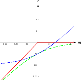
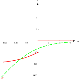
Figure 1: Plots of relative improvement r of accuracy (i.e.,
reduction of variance) depending on the ability ratio m after
considering the advisor’s advice using three different methods:
Choosing the better estimate (red plain), averaging both estimates
equally (blue dotted), and weighting the estimates according to
ability ratio (green dashed). Since r is measuring the change of
variance compared to the initial estimate, r<0 means an
improvement while r>1 means worsening of the initial
estimate. Both axes are in logarithmic scale.
Figure 2: Here, weighting uses the precise ability ratio m and choosing identifies the correct expert at 100%.
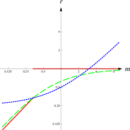
Figure 3: The judge overestimates her ability relative to that of the advisor by 200% (i.e., p = 3), resulting in imperfect weighting and, for some values of m, choosing the wrong estimate.
2.2 Imperfect weighting: The effect of errors in assessing the ability differences
As we have demonstrated in the last subsection, perfect weighting is superior to choosing and averaging. However, perfect weighting requires that the ability ratio between judge and advisor is known to the judge. Despite judges’ ability to differentiate between good and bad advice beyond chance level (e.g., Harvey and Fischer [1997], Harvey et al. [2000], Yaniv [2004], Yaniv and Kleinberger [2000]) exact knowledge of m is unlikely. Let us, accordingly, assume that m must be estimated by the judge and is, therefore, subject to errors or biases. In essence, regardless of whether such a mistake is systematic or not, the judge can either under- or over-estimate the true value of m, and we denote the degree to which the judge does so by the factor p. If p equals 1, the judge has a perfect representation of the ability ratio. In contrast, values greater than 1 indicate that the judge’s perception of the ability erroneously shift in his or her favor, whereas values smaller than 1 mean that the judge overestimates the ability of the advisor. Technically speaking, p varies misconception by either magnifying or dampening the ratio m. Thus, instead of (5) the judge’s final result reads as
x(p)=
pm
1+pm
xJ+
1
1+pm
xA
(6)
and the variance of x(p) is given by
σp2=
m2p2σJ2+σA2
(1+pm)2
(7)
In this case, the final estimate by weighting the two initial estimates differently might end up being worse than taking the simple average. This would happen if the ability ratio is (i) not very large and (ii) poorly estimated. The weighted mean might also end up being worse than choosing the better guess. This would happen if the competence ratio is actually large, but is perceived as small. To see the full picture we need to compare the relative improvements
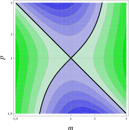
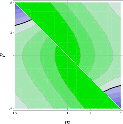
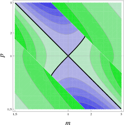
Figure 4: Contour plot of the relative difference k of averaging/weighting (a) and choosing/weighting (b). The two methods are equally efficient at the thick black lines. In the green region weighting is more efficient while in the blue region averaging (a) / choosing (b) are more efficient. Again, efficiency is measured in the reduction of variance compared to the initial estimate: if weighting reduces more variance than averaging/choosing, it is more efficient. At the thick black line, k=1. Contour lines represent steps of 10%, i.e., k=0.6,0.7,...,1.4,1.5
Figure 5: Averaging vs. weighting
Figure 6: Choosing vs. weighting
r=
variance of final guess
variance of initial guess
(8)
of the judge. Values smaller than 1 indicate that the error variance of the final estimates is smaller than that of the initial estimate, that is, the final estimates are more accurate. In contrast, if the final estimates are less accurate than the initial estimates, r will assume values greater than 1. We determine the expected values of r for the three advice-taking strategies as a function of the parameters m and p (except, for averaging, which does not depend on p). For averaging, we get
raveraging(m)=
σa2
σJ2
=
1
4
σJ2+σA2
σJ2
=
1+m
4
(9)
with the expected variance of averaging σa2=1/4(σJ2+σA2). For weighting, we get
rweighting(m,p)=
σp2
σJ2
=
m2p2 σJ2+σA2
(1+pm)2σJ2
(10)
=
m2p2
(1+pm)2
+
m
(1+pm)2
=
m(1+p2m)
(1+pm)2
(11)
For choosing, we first observe that rchoosing can only be either 1, or m. In the first case, the judge chooses her own estimate and therefore can neither improve nor worsen. In the latter case, the accuracy changes exactly by the competence ratio m. Essentially, the judge must guess whether m>1 or m<1. However, she knows only pm instead of m which gives
rchoosing(m,p)=
⎧
⎨
⎩
m,
if pm<1
1,
else
(12)
Obviously, the judge does not always identify the correct expert. This happens if either m is chosen despite m>1 (because pm<1) or of 1 is chosen despite m<1 (because pm>1). Essentially, these three r-functions tell us how much the judge improves or worsens her initial estimate by using either averaging, weighting or choosing.
In Figure 3, we show LogLog Plots1 with fixed p, p=1 (left panel) and p=3 (right panel) varying the ability ratio m. In line with the reasoning above, Figure 3(a) shows that if the judge can correctly assess the ability differences, weighting outperforms both averaging and choosing. However, as we can see in Figure 3(b), the relative performance of the three strategies differs for specific parameter regions. In our example, the judge overestimates her ability relative to that of the advisor by 200% (i.e., p=3). In this case, averaging outperforms weighting for small ability ratios, and choosing outperforms weighting if the advisor is substantially more accurate than the judge.
Next, we want to explore the full parameter space of m and p. To
this end, we need to compare the relative improvement in accuracy
obtained by the different strategies as a function of the model
parameters p and m. Specifically, we are interested in the
relative performance of weighting on one hand and either choosing or
averaging on the other (for an in-depth comparison of choosing and
averaging, see Soll and Larrick [2009]), which we denote as
kaveraging=
rweighting
raveraging
(13)
and
kchoosing=
rweighting
rchoosing
(14)
respectively. A value of k = 1 indicates that weighting and the comparison strategy (averaging or choosing) perform equally well whereas values of k > 1 indicate superior performance of weighting, and values of k < 1 indicate that the respective comparison strategy performs better. The target value k is represented by the shade in the contour plot spanned by the parameters m and p (see Figure 6). The bold line separating the blue and green regions is the iso-accuracy curve which indicates that the accuracy of the weighting strategy equals that of the comparison strategy (i.e., k = 1). For each subsequent line in the green area, k increases by 0.1, that is, the weighting-method performs 10% better than averaging/choosing, while in the blue area the opposite is true.
As can be seen in Figure 5, if there are ability
differences between judge and advisor and the judge has a rough
representation of these differences, weighting is superior to simple
averaging. In contrast, whenever the ability differences are small
and/or difficult to detect, judges will benefit more from
averaging. The accuracy differences between weighting and choosing are
more pronounced (see Figure 6). Obviously, the judge must
make extreme errors when assessing m in order for choosing to be the
better advice taking strategy. In addition, choosing can outperform
weighting only if correctly identifying the better estimate. This is
the case above the white diagonal in Figure 6 for
m > 1, and below the diagonal for m < 1. Note that the second
prerequisite creates an asymmetry in the results. This asymmetry is
rooted in the fact that choosing is heavily penalized if the judge
erroneously chooses the wrong estimate while weighting is much less
prone to such extreme errors because it still assigns some weight to
the more accurate judgment.
Our analysis so far revealed that weighting is quite a powerful
strategy when comparing it to either averaging or choosing. However,
one rationale that we can derive from Soll and Larrick’s (2009) PAR
model is that judges should switch between averaging and choosing in
order to maximize the accuracy of their final estimates. Specifically,
they should average when ability differences are small and/or
difficult to detect and choose when the opposite is true. An
interesting vantage point, then, is to compare weighting to a
combination of choosing and averaging.
2.3 Combining averaging and choosing
Let us assume that judges know when they should switch from averaging
to choosing based on their (potentially biased) perception of m. We
can easily compute this threshold by equating rchoosing and
raveraging
1+m
4
=1
(15)
⇔ m
=3
(16)
if, choosing one self, and
1+m
4
=m
(17)
⇔ m
=1/3
(18)
if choosing the advisor. Since the judge estimates m as pm, she
will change whenever pm = 3 or pm = 1/3. In other words, a
perfect application of the combined strategy implies that judges
average their initial estimates and the advice until they perceive the
initial estimates to be three times as accurate as the advice or vice
versa; if this threshold is passed, they choose the more accurate
estimate. If m is estimated without error (i.e., p = 1),
dynamically switching between choosing and averaging is a powerful
strategy. However, we have to take into account that if p ≠ 1,
choosing will not always be correct, since the judge may erroneously
choose the less accurate judgment. This flaw drastically reduces the
performance of the combined strategy, because choosing the wrong
expert has highly negative consequences.
Figure 7: Comparing weighting to the combination of choosing and averaging.
Figure 8: Relative improvement of accuracy (as in Fig.1) of weighting (green dashed) and the combined method (red plain), both for p = 3. Note that imperfect estimation of m leads to choosing the wrong judgment in a certain parameter regions.
Figure 9: Generalization of (a) by allowing for varying p (as in Fig. 2). In the green area, weighting is the better strategy, while in the blue area the combined method performs better. The contour lines denote increases or decreases in steps of 10%.
In order to compare weighting to the combined strategy of choosing and
averaging, we first determine the accuracy gains relative to the
initial estimates that would result from a combination of choosing and
averaging, rcombined. Figure 3 (left panel) compares the accuracy
ratios of the combined strategy as well as that of weighting as a
function of m and assuming that the judge is strongly overestimating
his or her own accuracy (p = 3). We next calculated the ratio of
the accuracy gain obtained by weighting and that obtained by the
combined strategy:
kcombined=
rweighting
rcombined
(19)
The right panel of Figure 3 shows kcombined as a function of m and p. The white lines denote the threshold at which judges switch from averaging to choosing based on their perception of the relative accuracy of judge and advisor (i.e., when the product pm is greater than 3 or smaller than 1/3). The bold lines, again, denote the iso-accuracy-curves. The analysis reveals some interesting findings. First, weighting is superior to the combined strategy in a wide range of situations. Second, the superiority of the weighting strategy is mostly due to the relatively weak performance of choosing. The problem is that the application of the combined strategy sometimes leads to choosing in situations in which averaging would outperform weighting but choosing does not. This happens when ability differences are small and difficult to assess (i.e., m close to 1 and p either very small or very large). Instances where the choosing part of the combined strategy performs better than the weighting strategy occur only for extreme competence differences outside of the parameter range of Figure 3.
3 Discussion
The aim of our theoretical analysis was to answer the question which advice-taking strategy judges in a judge-advisor system should utilize in order to maximize the accuracy of their revised estimates. Previous research has suggested that judges should average their initial estimates and the advice unless the difference in accuracy between the two estimates is large and easily identifiable; in such cases they should simply choose the more accurate estimate (Soll and Larrick [2009]). It is a mathematical fact that averaging two independent and unbiased estimates leads to, on average, more accurate judgments (e.g., Larrick and Soll [2006], Yaniv [2004]). However, if the error variance of the two judgments is unequal, there is an optimal weight of advice that produces combined estimates that are always equal or better than simple averaging with regards to accuracy. As a consequence, judges in a judge-advisor system would benefit the most from weighting the advice according to its accuracy relative to that of the judges’ initial estimate (Budescu [2006], Budescu and Yu [2006]). Similar to choosing the better estimate, the potential superiority of the weighting strategy compared to pure averaging comes at the cost of additional information, namely knowledge of the ability difference between judge and advisor.
If this ability difference is known, a weighting strategy is bound to be superior to both, averaging and choosing. Yet, it is rather unlikely that judges will be able to correctly recognize differences between their own and their advisor’s ability with perfect accuracy. Instead, previous research suggests that while judges have some ability to assess the relative quality of advice they frequently underestimate it (e.g., Harvey and Fischer [1997], Harvey et al. [2000], Yaniv and Kleinberger [2000]). In other situations, for example, when judges perceive the task as very difficult (Gino and Moore [2007]) or when they are very anxious, they are prone to overestimate the quality of the advice relative to that of their own initial estimates (Gino et al. [2012]). If judges’ assessment of the ability differences are subject to errors the resulting weighting strategy will result in less accurate judgments, and if these errors become too large, simple averaging turns out to be the better strategy. The fact that the averaging strategy can outperform weighting strategies that are based on erroneous weights has been previously documented in multi-cue judgments (Dawes [1979]), and the advantage of averaging increases as the number of cues grows. Hence, the first question we aimed to answer was under which conditions imperfect weighting outperforms averaging. To this end, we compared the expected performance of both strategies as a function of ability differences between judge and advisor as well as the accuracy of the judge when estimating these differences.
Our analysis revealed that imperfect weighting outperforms averaging
as long as there are at least moderate ability differences. This
performance advantage of the weighting strategy is rather robust
against moderate misperceptions of the ability differences. For
example, if the judge’s error was 50% larger than that of the
advisor, weighting is superior to averaging even if the judge under-
or overestimates the ability difference by 50%. Additionally, the
larger the ability differences become the more robust the weighting
strategy becomes against erroneous assessment of these differences. In
other words, averaging is likely to produce better estimates than
imperfect weighting only when ability differences are small and/or
difficult to detect.
We also compared an imperfect weighting strategy to imperfect
choosing, finding that the former outperformed the latter with very
few exceptions. Specifically, choosing was superior to weighting only
when there were large differences in accuracy which the judge
recognized but severely underestimated. The reason for this finding is
that the choosing strategy is insensitive to the magnitude of the
ability differences whereas the weighting strategy is not. Consider
the case where the advisor is much more accurate than the judge but
the judge erroneously perceives the advisor to be only slightly better
than him- or herself. In this case the judge will still correctly
identify the advisor as the expert, and because the actual difference
in expertise is large, choosing the advice will produce a rather good
result. In contrast, weighting will produce a final estimate that is
not too different from (but slightly superior to) the one obtained by
averaging because the difference in weights is bound to be
small. Based on the misperception of the ability differences, the
judge does not assign enough weight to the advice.
Finally, we compared imperfect weighting to a strategy that
dynamically switches from averaging to choosing when the (potentially
biased) perceived ability differences between judge and advisor become
large (Soll and Larrick [2009]). Our analysis revealed that weighting
is superior to the combined strategy in a wide range of
situations. Interestingly, weighting is better than the combined
strategy mainly because the application of the combined strategy leads
judges to choose between estimates in situations where averaging would
outperform weighting. These situations are characterized by the judge
correctly recognizing whether the advisor is more competent than him-
or herself or vice versa, but at the same time greatly overestimating
the ability differences. The interesting thing about those situations
is that simple averaging would have performed better than weighting,
but since the ability differences are perceived as too high, the
combined strategy must use choosing instead.
3.1 Implications and directions for future research
An important implication of our analysis is that weighting is a highly
effective strategy in advice taking. This finding extends previous
research on judgmental aggregation. So far, the respective literature
has unanimously supported averaging as the most robust strategy when
it comes to utilizing the wisdom of the crowds (e.g., Clemen
[1989], Davis-Stober et al. [2014], Smith and Wallis [2009]). In
addition, some recent studies showed that a combination of choosing
and averaging can outperform mere averaging. In these studies, the
average of all individuals judgments were compared to the average of a
subset comprised of the most accurate judgments (Davis-Stober et
al. [2014]) or those judgments supposedly more accurate based on
incomplete historic data (Mannes et al. [2014]). In contrast,
differential weighting of the individual judgments usually performs
worse than simple averaging (e.g., Dawes [1979], Genre et
al. [2013]). The reason for this is the inflation of errors when
estimating the optimal weights of a large set of individual judgments
(Smith and Wallis [2009]). However, in the context of the
judge-advisor dyad, the judge needs only estimate one parameter when
estimating the optimal weight of advice. Therefore, the risk of error
inflation is minimal and, as a consequence, weighting becomes a
powerful strategy.
Furthermore, the fact that participants in previous studies adhered to a weighting strategy in a substantial number of trials (Soll and Larrick [2009], Soll and Mannes [2011]) as well as its potential superiority to averaging highlight its importance when studying advice taking. Whereas the PAR model suggests that judges should engage in averaging in case of small or difficult to detect ability difference and rely on choosing otherwise, our analysis makes a partially different statement. In case of small and difficult to detect ability differences, averaging is still the best option. However, in case the ability differences become larger and easier to detect, judges should attempt to weight the two judgments by perceived accuracy instead of choosing between the two. Interestingly, weighting the two estimates by their perceived accuracy allows judges to mimic an aggregation strategy that has proven to be very effective if three or more judgments are involved, namely taking the median. Research on group judgment (Bonner et al. [2004], Bonner et al. [2007], Bonner and Baumann [2008]) suggests that the way in which groups or judges combine the individual estimates is best described by the median or similar models that discount outliers. The same is true when judges combine several independent judgments (Yaniv [1997]) or receive advice from multiple advisors (Yaniv and Milyavsky [2007]). Importantly, the median strategy outperforms the average because it discounts extreme judgments which are usually less accurate. Naturally, in the JAS with only one advisor, the median is per definition, equal to the mean, but assigning more weight to the more accurate judgment, even if the weight is not optimal due to misperceptions of the ability differences, also leads to discounting the less accurate judgments.
Our theoretical analysis does not only provide a normative framework to compare the expected performance of different advice taking strategies. It also allows to evaluate the effectiveness of judges’ advice taking strategies. Similar to Soll and Larrick’s (2009) empirical analysis, our model provides performance baselines against which to compare the de facto improvements in accuracy between judges’ initial and final estimates. Soll and Larrick’s analyses already showed that in the majority of the cases frequent averagers outperformed frequent choosers. An interesting question would, then, be whether or under which conditions frequent weighting can outperform frequent averaging.
Finally, a potential venue for further developing our model would be to include biased judgments. In our theoretical analysis, we made the simplifying assumption that there is no systematic bias in the judge’s and advisor’s estimates. Incorporating systematic biases of judge and advisor will necessarily make the model more complex, but it may be worthwhile if it allows us to draw conclusions about the relative performance of weighting, choosing and averaging in a wider range of decision situations.
3.2 Conclusion
Advice taking is not only an integral part of our daily social reality
but also one of the most effective ways to increase the quality of our
judgments and decisions. In order to make the best use of the wisdom
of others, we need a thorough understanding of how well we utilize
advice depending on its quality. An elegant way to provide answers to
this question is provided by normative models of advice taking. We
built on and extended the most prominent normative model of advice
taking and, by doing so, furthered our understanding of how effective
different advice taking strategies are in different situations. More
importantly, however, normative modeling allows us to detect and,
ultimately intervene against, deviations from optimal strategies, that
is, they can help us utilize the benefits of advice to its full
effect.
Bonaccio, S. and Dalal, R. S. (2006).
Advice taking and decision-making: An integrative literature review,
and implications for the organizational sciences.
Organizational Behavior and Human Decision Processes,
101(2):127--151.
[ bib ]
Bonner, B. L. and Baumann, M. R. (2008).
Informational intra-group influence: the effects of time pressure and
group size.
European Journal of Social Psychology, 38(1):46--66.
[ bib ]
Bonner, B. L., Gonzalez, C. M., and Sommer, D. (2004).
Centrality and accuracy in group quantity estimations.
Group Dynamics: Theory, Research, and Practice, 8(3):155.
[ bib ]
Bonner, B. L., Sillito, S. D., and Baumann, M. R. (2007).
Collective estimation: Accuracy, expertise, and extroversion as
sources of intra-group influence.
Organizational Behavior and Human Decision Processes,
103(1):121--133.
[ bib ]
Budescu, D. (2006).
Confidence in aggregation of opinions from multiple sources,
pages 327--352.
New York, NY: Camridge University Press.
[ bib ]
Budescu, D. V. and Yu, H.-T. (2006).
To bayes or not to bayes? A comparison of two classes of models of
information aggregation.
Decision analysis, 3(3):145--162.
[ bib ]
Clemen, R. T. (1989).
Combining forecasts: A review and annotated bibliography.
International Journal of Forecasting, 5(4):559--583.
[ bib ]
Davis-Stober, C. P., Budescu, D. V., Dana, J., and Broomell, S. B. (2014).
When is a crowd wise?
Decision, 1(2):79.
[ bib ]
Dawes, R. M. (1979).
The robust beauty of improper linear models in decision making.
American Psychologist, 34(7):571.
[ bib ]
Einhorn, H. J., Hogarth, R. M., and Klempner, E. (1977).
Quality of group judgment.
Psychological Bulletin, 84(1):158.
[ bib ]
Genre, V., Kenny, G., Meyler, A., and Timmermann, A. (2013).
Combining expert forecasts: Can anything beat the simple average?
International Journal of Forecasting, 29(1):108--121.
[ bib ]
Gino, F., Brooks, A. W., and Schweitzer, M. E. (2012).
Anxiety, advice, and the ability to discern: feeling anxious
motivates individuals to seek and use advice.
Journal of Personality and Social Psychology, 102(3):497.
[ bib ]
Gino, F. and Moore, D. A. (2007).
Effects of task difficulty on use of advice.
Journal of Behavioral Decision Making, 20(1):21--35.
[ bib ]
Gino, F. and Schweitzer, M. E. (2008).
Blinded by anger or feeling the love: how emotions influence advice
taking.
Journal of Applied Psychology, 93(5):1165.
[ bib ]
Harvey, N. and Fischer, I. (1997).
Taking advice: Accepting help, improving judgment, and sharing
responsibility.
Organizational Behavior and Human Decision Processes,
70(2):117--133.
[ bib ]
Harvey, N., Harries, C., and Fischer, I. (2000).
Using advice and assessing its quality.
Organizational Behavior and Human Decision Processes,
81(2):252--273.
[ bib ]
Larrick, R. P. and Soll, J. B. (2006).
Intuitions about combining opinions: Misappreciation of the averaging
principle.
Management science, 52(1):111--127.
[ bib ]
Mannes, A. E., Soll, J. B., and Larrick, R. P. (2014).
The wisdom of select crowds.
Journal of Personality and Social Psychology, 107(2):276.
[ bib ]
Minson, J. A., Liberman, V., and Ross, L. (2011).
Two to tango: Effects of collaboration and disagreement on dyadic
judgment.
Personality and Social Psychology Bulletin, page
0146167211410436.
[ bib ]
Minson, J. A. and Mueller, J. S. (2012).
The cost of collaboration why joint decision making exacerbates
rejection of outside information.
Psychological Science, 23(3):219--224.
[ bib ]
Smith, J. and Wallis, K. F. (2009).
A simple explanation of the forecast combination puzzle*.
Oxford Bulletin of Economics and Statistics, 71(3):331--355.
[ bib ]
Sniezek, J. A. and Buckley, T. (1995).
Cueing and cognitive conflict in judge-advisor decision making.
Organizational Behavior and Human Decision Processes,
62(2):159--174.
[ bib ]
Sniezek, J. A., Schrah, G. E., and Dalal, R. S. (2004).
Improving judgement with prepaid expert advice.
Journal of Behavioral Decision Making, 17(3):173--190.
[ bib ]
Soll, J. B. and Larrick, R. P. (2009).
Strategies for revising judgment: How (and how well) people use
others' opinions.
Journal of Experimental Psychology: Learning, Memory, and
Cognition, 35(3):780.
[ bib ]
Soll, J. B. and Mannes, A. E. (2011).
Judgmental aggregation strategies depend on whether the self is
involved.
International Journal of Forecasting, 27(1):81--102.
[ bib ]
Yaniv, I. (1997).
Weighting and trimming: Heuristics for aggregating judgments under
uncertainty.
Organizational Behavior and Human Decision Processes,
69(3):237--249.
[ bib ]
Yaniv, I. (2004).
The benefit of additional opinions.
Current Directions in Psychological Science, 13(2):75--78.
[ bib ]
Yaniv, I. and Kleinberger, E. (2000).
Advice taking in decision making: Egocentric discounting and
reputation formation.
Organizational Behavior and Human Decision Processes,
83(2):260--281.
[ bib ]
Yaniv, I. and Milyavsky, M. (2007).
Using advice from multiple sources to revise and improve judgments.
Organizational Behavior and Human Decision Processes,
103(1):104--120.
[ bib ]
Let us assume that the estimates of both judge and advisor are independent and drawn from a normal distribution centered on the true value xT with variances σJ2 and σA2. Since xJ and xA are drawn from independent distributions, the density function is given by
We compare the weighted average (2) with the arithmetic (non-weighted) average x.
x=
1
2
(xA+xB)
(26)
First, let us recall that for any random variable X and a real number a holds
Var(aX)=a2Var(X)
(27)
Further, if X and Y follow independent Gaussian distributions (µX,σX2) and (µY,σY2), respectively, then also X+Y follows a Gaussian distribution with expected value µX+Y=µY+µY and variance σX+Y2=σX2+σY2.
Now we look at the distributions of x and x. Since they are both linear transformations of xJ and xA we can directly apply the above two rules. Thus, x and x follow a Gaussian distribution with expected value xT and the respective variances
σw2
=
σJ2σA2
σJ2+σA2
(28)
σa2
=
1
4
(σJ2+σA2)
(29)
where σw2 is the variance of the weighted mean and σa2 is the variance of the arithmetic mean. Then σw ≤ σa with equality only if σA=σB, because
Our model differs from the PAR
model in three aspects. First, whereas both the PAR and our model
assume normally distributed estimates, our model makes the
additional assumption of unbiased estimates for the sake of
simplicity. Second, the error measures differ: while the PAR model
measures judgment errors in terms of the mean absolute error, we
chose the mean squared error due to its favorable mathematical
properties. Note, that the choice of error measures can change
the results only quantitatively, but not qualitatively. That is, if one
aggregation strategy is superior to another it is so regardless of
the error measure applied. Finally, our models differ in the way the
recognition of ability differences is operationalized. Whereas the
PAR model models it in terms of a correlation between two binary
variables (which dyad member is more competent vs. which dyad member
does the judge perceive to be more competent), our model treats the
recognition of relative expertise as a continuous variable. This
variable not only states which dyad member is more accurate but also
quantifies the magnitude of the ability difference. The latter is
necessary in order to determine the (perceived) optimal weight of
advice.
If, instead of deriving the optimal method theoretically, we would restrict ourselves on the method of assigning linear weights (weighting) to xA and xJ, we could compute the optimal weight by simply optimizing the equation σw2=(1−w)2σJ2+w2σA2 with respect to σw2.
Institute of Psychology, Georg-August-University Goettingen
Portions of this research were presented at the 2010 Association for
Psychological Science annual convention. The authors thank Jay Hull,
Bertram Malle, and the Moral Psychology Research Group for their
helpful comments. Discussions with Dirk Semmann and Stefan
Schulz-Hardt are gratefully acknowledged. The research is partly
funded by the German Initiative of Excellence of the German Science
Foundation (DFG). We thank Robin Hogarth and two anonymous reviewers
for helpful comments.
This paper is dedicated to Nicola Knight, whose untimely death
saddened us all. Nicola contributed much inspiration and hard work
during the design phase of this study.
A brief remark for readers unfamiliar with LogLog plots: Since the variables m and r that we wish to plot are relations, we need to scale the axes accordingly. A value of m = 0.5 means that the judge is twice as good as the advisor while m = 2 means that the advisor is twice as good as the judge. Similarly for m = 0.1 and m = 10. This means that we need to treat the two intervals (0; 1) and (1;∞) equally. Further, we must center the plot around 1 instead of 0 because a value of m = 1 indictaes equal accuracy of judge and advisor. This is accomplished by Log(-arithmic) scaling. Double logarithmic scaling (i.e., LogLog Plots) scales both axes logarithmically.