The average laboratory samples a population of 7,300 Amazon Mechanical Turk workers
Neil Stewart* Christoph Ungemach# Adam J. L. Harris$ Daniel M. Bartelsº Ben R. Newell Gabriele Paolacci|| Jesse Chandler**
Using capture-recapture analysis we estimate the effective size of the active Amazon Mechanical Turk (MTurk) population that a typical laboratory can access to be about 7,300 workers. We also estimate that the time taken for half of the workers to leave the MTurk pool and be replaced is about 7 months. Each laboratory has its own population pool which overlaps, often extensively, with the hundreds of other laboratories using MTurk. Our estimate is based on a sample of 114,460 completed sessions from 33,408 unique participants and 689 sessions across seven laboratories in the US, Europe, and Australia from January 2012 to March 2015.
Keywords: Amazon Mechanical Turk, MTurk, capture-recapture, population size.
1 Introduction
Amazon Mechanical Turk (MTurk) offers a large on-line workforce who
complete human intelligence tasks (HITs). As experimenters, we can
recruit these MTurk workers to complete our experiments and surveys
(for a review, see Paolacci and Chandler, 2014). This is exciting,
because the MTurk population is more representative of the population
at large, certainly more representative than an undergraduate sample,
and produces reliable results at low cost (Behrend et al. [2011], Berinsky et al. [2012], Buhrmester et al. [2011], Paolacci et al. [2010], Woods et al. [2015]). MTurk reports having 500,000 registered workers from 190 countries. MTurk workers are used in psychology, economics, and political science, with classic findings replicated in all three domains (Berinsky et al. [2012], Goodman et al. [2013], Horton et al. [2011], Klein et al. [2014], Mullinix et al. [2014], Paolacci et al. [2010]).
There are hundreds of MTurk studies: The PsychARTICLES database, which searches the full text of articles in APA journals, reports 334 articles with the phrase “MTurk” or “Mechanical Turk”, all in the last five years. There are 82 articles in the (non-APA) journal Judgment and Decision Making and 99 articles in the (non-APA) journal Psychological Science with these phrases in the full text, again all in the last five years (see Woods et al. [2015]). Exactly half of these articles have appeared since January 2014—that is, in about the last year the total number of articles mentioning MTurk has doubled. Google Scholar gives 17,600 results for this search and 5,950 articles for 2014 alone. The anonymity and speed of MTurk data collection, and the volume of papers makes the pool of workers seem limitless. When a laboratory conducts a study on MTurk, how many participants are in the population from which it is sampling? The population size matters for planning a series of experiments, considerations about participant naïveté, and running similar experiments or replications across laboratories.
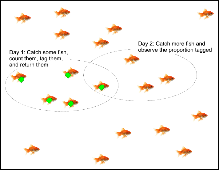
To address this question we used capture-recapture analysis, a method frequently used in ecology and epidemiology to estimate population sizes (Seber [1982]). The logic of capture-recapture analysis is illustrated by the Lincoln-Petersen method: To estimate the number of fish in a lake, make two fishing trips. On the first trip catch and mark some fish before returning them. On the second trip, catch some fish and observe the proportion that are marked. The total number of unmarked fish in the lake can be estimated by extrapolating the proportion of marked and unmarked fish caught on the second trip to the (known) number of fish marked on the first trip and the (unknown) number of unmarked fish in the lake. You don’t need to catch all of the fish in the lake to estimate how many there are.
We used an open-population capture-recapture analysis (Cormack [1989]), which allows for MTurk workers to enter and leave the population. As we found moderate turnover rates, these open-population models are more appropriate than the closed-population models (Otis et al. [1978]). We use the Jolly-Seber open-population model, which allows us to estimate the population size, rates of survival from one period to the next, and new arrivals to the population (Cormack [1989], Rivest and Daigle [2004]). A tutorial on the application of capture-recapture models is given in the Appendix.
Below we apply this capture-recapture analysis to the MTurk population, but this method could be used to estimate the size of any human population by sampling people several times (Fisher et al. [1994], Laporte [1994]). The raw data for these analyses come from the batch files which one can download from the MTurk requester web pages. These batch files contain, among other things, a WorkerId which is a unique identifier for each worker and that allows us to track workers across experiments and laboratories. To preempt the results, our laboratories are sampling from overlapping pools, each pool with fewer than 10,000 workers.
2 The laboratories
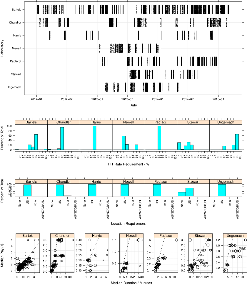
We have pooled data from our seven laboratories, each with a separate MTurk account. Our laboratories are based in the US, UK, the Netherlands, and Australia. There were 33,408 unique participants or, in the language of MTurk, workers. These workers completed 114,460 experimental sessions or HITs. HITs were run in 689 different batches, with one experiment often run in multiple batches. The HITs were short experiments, often in the domain of judgment and decision making.
The top panel in Figure 1 shows how the dates of sessions for each lab. The sessions took place between 7 January 2012 and 3 March 2015.
The middle rows of Figure 1 show requirements of participants in terms of HIT acceptance history and geographical location. As is typical for experimental research on MTurk, all HITs were opened beyond “Master” level workers. Only Stewart opened HITs to significant proportion of workers from outside the US and only Stewart allowed a non-trivial fraction of workers with HIT approval rates below 90%.
The bottom panel of Figure 1 plots median pay
against duration for each experimental session. Duration is likely to
be noisy because people sometimes accept the HIT after completing a
task, sometimes accept a HIT and take a break before completing the
task, and sometimes complete other tasks simultaneously. Across
laboratories, median pay was $0.35 and median duration was 4.4
minutes. The median hourly wage was $5.54 though this will be an
underestimate if durations are overestimated. (The US federal minimum
is now $7.25.)
Figure 1: The details of timing, HIT acceptance and location requirements, and pay and duration across the seven labs. The first row shows the timing of the experiments by laboratory. A dot, jittered vertically, represents a single HIT. The second and third rows show the differences between laboratories in HIT acceptance rates and location requirements for participation. The final row shows scatter plots of the median pay against duration for each experiment. Each circle is a batch and its area is proportional to the number of HITs. The dashed line is the $7.25 per hour US federal minimum wage, with batches under the line paying less. Note, scales differ over panels.
3 The size of the MTurk population
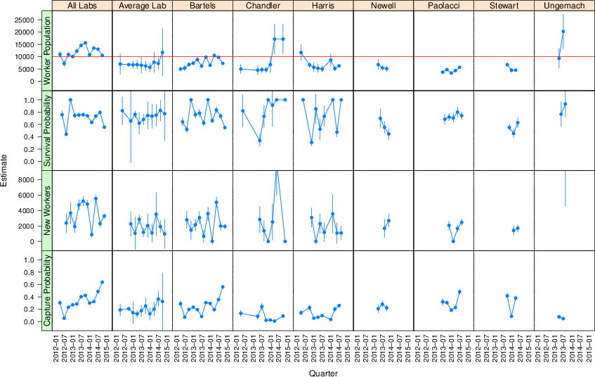
We included all HITs in our open-population analysis, except HITs where participants were invited to make multiple submissions and HITs were participation was only open to those who had taken part in a previous HIT. This removed 19% of HITs. These are the only exclusions. In estimating the open-population model, we treated each of the 13 quarter years from January 2012 to March 2015
as a capture opportunity. We fitted the model separately for each laboratory.
Figure 2 displays the estimates from the open population analysis. Each column is for a different laboratory. Each row displays the estimate for different parameters across the 13 quarters. In the Jolly-Seber model estimates for the first and last quarter are not available. (See the Appendix for details on this issue and also Baillargeon and Rivest [2007], Cormack [1989].)
The top row contains the estimates of the size of the MTurk population each laboratory can reach in each quarter, which is our primary interest. Estimates of the worker population size vary across time and laboratories, but estimates for individual labs are nearly always below 10,000 in every quarter. Note, this estimate is of the pool from which the laboratory sampled, not the number of workers actually sampled.
The leftmost column contains an estimate for the joint reach of all seven laboratories, where all the data are pooled as if they came from one laboratory. Our seven laboratories have a joint reach of between about 10,000 and 15,000 unique workers in any quarter (average 11,800).
The second column contains estimates for a hypothetical laboratory, labelled “Average Lab”, derived by combining the estimates from each of the seven laboratories using a random effects meta analysis (Cumming [2014]). There is considerable heterogeneity across laboratories (median I2 = 96%), though we leave exploring these differences to later experimental investigation. Effectively, the meta analysis is our best estimate at the reach of an unknown eighth laboratory, which could be yours. The average over time of the population size we expect this unknown laboratory to reach is about 7,300 unique workers.
Figure 2: Open population analysis results. Error bars are the extent of 95% confidence intervals.
The second row gives estimates of the probability that a worker in the population survives, or persists, from one quarter to the next. The random effects meta analysis gives a mean estimate of .74. This corresponds to a worker half-life of about 7 months—the time it takes for half of the workers present in one quarter to have left.
The third row gives estimates of the number of new workers arriving in the population sampled by a laboratory. The random effects meta analysis gives a mean estimate of about 1,900 new workers arriving each quarter for the average laboratory. For our combined laboratories, the mean estimate is 3,500 new workers arriving each quarter.
The bottom row gives estimates of the probability that workers will be sampled in the laboratory each quarter. Estimates vary across labs and time, and will be determined by the number of HITs offered, given almost all HITs offered are taken.
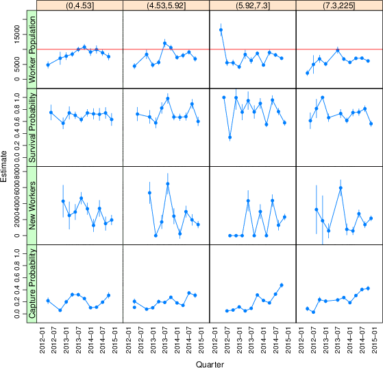
3.1 Pay
Buhrmester et al. [2011] found that increasing pay rates increased the rate at which workers were recruited but did not affect data quality. We found that paying people more does not increase the population available—at least not within the ranges our laboratories covered. Figure 3 repeats the Jolly-Seber open population modeling, but splitting HITs by hourly pay rate quartile instead of laboratory. The mean population estimate, averaged across quarters, decreased from 8,400 95% CI [8,100–8,800] for the lowest rates of pay to 6,200 95% CI [5,800–6,500] for the highest rates of pay. An analysis with absolute pay rather than pay rate also found no positive effect of pay on the population estimate.
Figure 3: Open population analysis results for different hourly rates of pay. Column headings give the ranges of pay rates for the four quartiles in the distribution of hourly pay. Error bars are the extent of 95% confidence intervals.
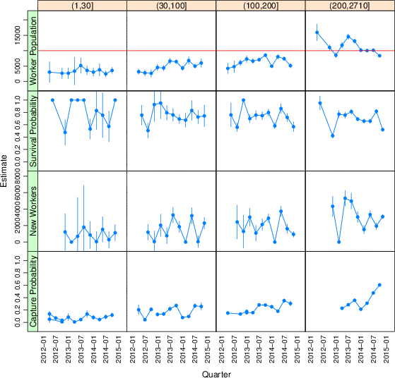
3.2 Batch size
Running batches in larger sizes does increase the size of the population available. Figure 4 repeats the Jolly-Seber open population modeling, but splitting HITs by the size of the quota requested when the batch was posted. Population estimates increase from 3,400 95% CI [2,600–4,100] for the smallest batches to 11,400 95% CI [11,000–11,700] for the largest batches from our combined laboratories.
Figure 4: Open population analysis results for different size batches. Column headings give the ranges of batch sizes for the four quartiles in the distribution of batch sizes. Error bars are the extent of 95% confidence intervals.
3.3 Robustness of the open population estimate
The Jolly-Seber model we estimate does not accommodate heterogeneity in the capture probability across workers. By examining the residuals we find captures in 10 or more quarters are more frequent than the Jolly-Seber model fit predicts. This means that there are some individuals who are particularly likely to be captured, perhaps reflecting the tendency for some participants to be especially interested in completing surveys, both on MTurk (Chandler et al. [2013]) and in other online nonprobability panels (Hillygus et al. [2014]). Thus we repeated the analysis excluding the individuals caught in 10 or more of the 13 quarters (34% of workers). The logic is that the individuals never caught—which is what we need to estimate to get the population total, given we have actually counted everyone else—are most like those caught rarely. The population estimate is, however, little affected by this exclusion. For example, the estimate of the reach of our combined laboratories increases slightly from 11,800 to 12,400.
We also reran the open-population estimation restricting the analysis to US workers with a HIT acceptance rate requirement of greater than 80%, which is the modal requirement across our seven labs.
The estimate of the reach of our combined laboratories decreased slightly from 11,800 to 10,900 per quarter. The number of new workers for our combined laboratories decreased from 3,500 to to 3,200 per quarter. Survival rates and capture probabilities are virtually identical.
Though we have not done so here, we could have modeled the heterogeneity in capture probability directly. We could also have used nested models to allow for migration between laboratories (Rivest and Daigle [2004]), which also deals with heterogeneous capture probabilities.
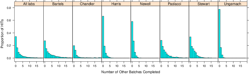
Figure 5: The distribution of the number of other batches completed within a laboratory.
4 Repeated participation
When you run a batch on MTurk, the default is to allow each worker to participate only once. But workers have very often completed many other batches on MTurk. They follow specific requesters or have a proclivity towards certain types of studies like psychology experiments (Chandler et al. [2013]). Figure 5 plots, for each laboratory, the distribution of the number of other batches completed. For example, in the Bartels laboratory, only 27% of HITs are from workers who did not complete any other HIT within the laboratory.
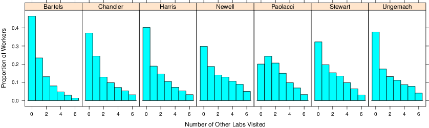
Figure 6 shows, for each laboratory, the distribution of the number of the other six laboratories visited by each worker. For example, in the Bartels laboratory, just under 50% of the workers did not visit any of the other six laboratories, and just over 50% visited at least one other laboratory.
Figure 6: The distribution of the number of other laboratories visited.
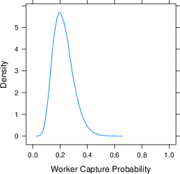
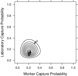
Figure 7 plots an estimate of the heterogeneity in the capture probabilities across laboratories and workers. The estimation is the random effects for worker and laboratory from a mixed effects logistic regression predicting capture. The plot is for a second capture in a named laboratory given an initial capture in a first laboratory. The probability that a particular worker gets caught in a particular lab is, on average, 0.21, with a 95% highest density interval of [0.08–0.48] for workers and [0.06–0.53] for laboratories. These capture probabilities can be used to estimate the probability of various capture history scenarios.
Figure 7: The joint distribution of worker and laboratory capture probabilities, together with marginal distributions.
Together with the population estimates, we can say that the average laboratories can access a population of about 7,300 workers, and that this population is shared in part with other laboratories around the world.
5 A simple replication
Casey and Chandler ran two large HITs simultaneously from their respective MTurk accounts between the 27th March and 9 May 2015 (Casey et al. [2015]). HITs were open to US workers with approval rates of 95% and over 50 HITs completed. Casey’s HIT was advertised as a 2-minute survey “about yourself” paying $0.25–$0.50. Chandler’s HIT was advertised as a 13-minute survey on “effective teaching and learning”, paying $1.50. Some workers took both HITs and this overlap allows us to estimate a simple closed-population capture-recapture model. With only two capture occasions, we cannot use an open-population model, but the HITs ran over a sufficiently short window that the coming and going of workers will not be large. Of the 11,126 workers captured in total, 8,111 took part in only Casey’s HIT, 1,175 took part in only Chandler’s HIT and 1,839 took part in both HITs. Given the asymmetry in the numbers caught in each lab, it is appropriate to allow for heterogeneity in capture probabilities in each lab. This Mt model is described in the Appendix. With only two capture opportunities, this model is saturated and is the most complex model we can estimate. The population estimate is 16,306 95% CI [15,912, 16,717]. This estimate is a little larger than the estimate based on the largest HITs from our seven labs reported in Section 3.2, but then the HITs were larger than anything we ran in our seven labs and, as we describe above, larger HITs reach a greater population. Overall, this independent estimate is in line with out seven-labs estimate.
6 Discussion
Our capture-recapture analysis estimates that, in any quarter year, the average laboratory can reach about 7,300 workers. In each quarter year, 26% of workers retire from the pool and are replaced with new workers. Thus the population that the average laboratory can reach only a few times larger than the active participant pool at a typical university (course-credit pools tend to have quite high uptake), with a turnover rate that is not dissimilar to the coming and going of university students. While the exact estimate will probably vary in the future, our message about the magnitude of the population available for the average laboratory—which is perhaps surprisingly small—is likely to remain valid given the stability of arrivals and survival rates.
Our estimates of the size of the population each laboratory is
sampling from is of the same order as Fort, Adda, and Cohen’s
[2011] estimate that 80% of HITs are completed by
3,011 to 8,582 workers, and that there are 15,059 to 42,912 workers in
total. In their estimate Fort et al. first construct an estimate for
the total number of HITs posted on MTurk each week by using a count of
the number of HITs lasting more than one hour from
http://mturk-tracker.com, adjusted by a multiple of 5 to get an
estimate the total number of HITs of any duration. Then they combine
this estimate with survey results from 1,000 workers self reporting
the number of HITs they complete per week and a blog post
(http://groups.csail.mit.edu/uid/deneme/?p=502) giving the
distribution of HITs per worker. Our estimates may differ for two
reasons. First, Fort et al.’s estimate depends on the accuracy of the
guestimate of the fraction of HITs that are greater than one hour and
on the accuracy of the worker self-reports. Second, our
capture-recapture analysis estimates the population available to our
laboratories, which will be a subset of the total population as we
select workers by location and HIT acceptance history, and workers
select our HITs or not. Thus our estimate is of the number of workers
available to researchers while Fort et al.’s is of the total number of
workers using MTurk.
Our findings about workers participating in multiple experiments
within a laboratory are broadly in line with earlier research that
demonstrates that workers participate in many different HITs within
the same laboratory
(Berinsky et al. [2012], Chandler et al. [2013]). We extend these
findings by demonstrating that workers are also likely to complete
experiments for many different laboratories. For example, of the
workers we captured, 36% completed HITs in more than one
laboratory. Of course, given we are only seven of a much larger set of
scientists using MTurk, it is extremely likely that our workers have
also taken part in many other experiments from other laboratories.
A growing body of research has illustrated the potential consequences
of non-naïveté. Many workers report having taken part in common
research paradigms (Chandler et al. [2013]). Experienced
workers show practice effects which may inflate measures of ability or
attentiveness to trick questions
(Chandler et al. [2013], Glinski et al. [1970], Hauser and Schwarz [2015]). Cooperation
in social games on MTurk has declined, perhaps as the result of too
much experience or learning
(Mason et al. [2014], Rand et al.). Participants
often conform to demand characteristics (Orne [1962]), and MTurk
workers may infer demands, correctly or otherwise, from debriefings
from earlier experiments. may Workers also have been previously
deceived, a key concern in behavioral economics
(Hertwig and Ortmann [2001]).
Thus there is a commons dilemma—your study may be improved by adding
classic measures or including deception, but subsequent studies may be
adversely affected. Participants previously exposed to an experiment
tend to show smaller effect sizes the second time
(Chandler et al. [2015]). If non-overlapping
samples are required, a relatively short series of experiments could
exhaust the MTurk population. For example, using 1,000 workers to
estimate a difference in a proportion gives a confidence interval .12
wide or, equivalently, an interval on d .28 wide. So replications by
other laboratories, which necessarily require larger sample sizes
(Simonsohn [2013]), may be hard and require a delay to allow new
workers to enter the pool.
We also observed considerable heterogeneity in the estimates of available workers across pools, suggesting that researcher practices can influence the amount of workers available to them. Many factors differ across our laboratories—such as the description of tasks, duration, posting time, requester reputation, or even just randomness in early update of HITs (Salganik et al. [2006])—and so experimental manipulation of these factors is required to make causal claims. However, we can offer two insights. We found that increasing pay did not increase the population available, but that running HITs in larger batches did. Both findings are consistent with more active workers seeking HITs quickly, crowding out other workers.
There are not that many people taking part in experiments on MTurk—about two orders of magnitude fewer than the 500,000 workers headlined by Amazon. We estimate that, if your laboratory used the MTurk population, you were sampling from a population of about 7,300 workers.
References
Baillargeon, S. and Rivest, L.-P. (2007).
Rcapture: Loglinear models for capture-recapture in R.
Journal of Statistical Software, 19.
[ bib |
.pdf ]
Behrend, T. S., Sharek, D. J., Meade, A. W., and Wiebe, E. N. (2011).
The viability of crowdsourcing for survey research.
Behavior Research Methods, 43:800--813.
[ bib |
DOI ]
Berinsky, A. J., Huber, G. A., and Lenz, G. S. (2012).
Evaluating online labor markets for experimental research:
Amazon.com's Mechanical Turk.
Political Analysis, 20:351--368.
[ bib |
DOI ]
Buhrmester, M., Kwang, T., and Gosling, S. D. (2011).
Amazon's Mechanical Turk: A new source of inexpensive, yet
high-quality, data?
Perspectives On Psychological Science, 6:3--5.
[ bib |
DOI ]
Casey, L., Chandler, J., Levine, A. S., Proctor, A., and Strolovitch, D.
(2015).
Demographic characteristics of a large sample of us workers.
[ bib ]
Chandler, J., Mueller, P., and Ipeirotis, P. G. (2013).
Nonnaïveté among Amazon Mechanical Turk workers:
Consequences and solutions for behavioral researchers.
Behavior Research Methods.
[ bib |
DOI ]
Chandler, J., Paolacci, G., Peer, E., Mueller, P., and Ratliff, K. (2015).
Using non-naïve participants can reduce effect sizes.
Psychological Science, 26:1131--1139.
[ bib |
DOI ]
Cormack, R. M. (1989).
Log-linear models for capture recapture.
Biometrics, 45:395--413.
[ bib |
DOI ]
Cumming, G. (2014).
The new statistics: Why and how.
Psychological Science, 25:7--29.
[ bib |
DOI ]
Fisher, N., Turner, S., Pugh, R., and Taylor, C. (1994).
Estimating the number of homeless and homeless mentally ill people in
north east Westminster by using capture-recapture analysis.
British Medical Journal, 308:27--30.
[ bib ]
Fort, K., Adda, G., and Cohen, K. B. (2011).
Amazon Mechanical Turk: Gold mine or coal mine?
Computational Linguistics, 37:413--420.
[ bib |
DOI ]
Francis, C. M., Barker, R. J., and Cooch, E. G. (2013).
Modeling demographic processes in marked populations: Proceedings of
the EURING 2013 analytical meeting [Special Issue].
Ecology and Evolution, 5.
[ bib |
DOI ]
Glinski, R. J., Glinski, B. C., and Slatin, G. T. (1970).
Nonnaivety contamination in conformity experiments: Sources, effects,
and implications for control.
Journal of Personality and Social Psychology, 16:478--485.
[ bib |
DOI ]
Goodman, J. K., Cryder, C. E., and Cheema, A. (2013).
Data collection in a flat world: The strengths and weaknesses of
mechanical turk samples.
Journal of Behavioral Decision Making, 26:213--224.
[ bib |
DOI ]
Hauser, D. J. and Schwarz, N. (2015).
Attentive turkers: Mturk participants perform better on online
attention checks than subject pool participants.
Behavior Research Methods.
[ bib |
DOI ]
Hertwig, R. and Ortmann, A. (2001).
Experimental practices in economics: A methodological challenge for
psychologists?
Behavioral and Brain Sciences, 24:383--451.
[ bib ]
Hillygus, D. S., Jackson, N., and Young, M. (2014).
Professional respondents in non-probability online panels.
In Callegaro, M., Baker, R., Lavrakas, P., Krosnick, J., Bethlehem,
J., and Gritz, A., editors, Online panel research: A data quality
perspective, pages 219--237. Wiley, West Sussex, UK.
[ bib ]
Horton, J. J., Rand, D. G., and Zeckhauser, R. J. (2011).
The online laboratory: Conducting experiments in a real labor market.
Experimental Economics, 14:399--425.
[ bib |
DOI ]
Klein, R. A., Ratliff, K. A., Vianello, M., Adams, Reginald B., J., Bahnik, S.,
Bernstein, M. J., Bocian, K., Brandt, M. J., Brooks, B., Brumbaugh, C. C.,
Cemalcilar, Z., Chandler, J., Cheong, W., Davis, W. E., Devos, T., Eisner,
M., Frankowska, N., Furrow, D., Galliani, E. M., Hasselman, F., Hicks, J. A.,
Hovermale, J. F., Hunt, S. J., Huntsinger, J. R., I. Jzerman, H., John,
M.-S., Joy-Gaba, J. A., Kappes, H. B., Krueger, L. E., Kurtz, J., Levitan,
C. A., Mallett, R. K., Morris, W. L., Nelson, A. J., Nier, J. A., Packard,
G., Pilati, R., Rutchick, A. M., Schmidt, K., Skorinko, J. L., Smith, R.,
Steiner, T. G., Storbeck, J., Van Swol, L. M., Thompson, D., van 't Veer,
A. E., Vaughn, L. A., Vranka, M., Wichman, A. L., Woodzicka, J. A., and
Nosek, B. A. (2014).
Investigating variation in replicability: A “many labs” replication
project.
Social Psychology, 45:142--152.
[ bib |
DOI ]
Laporte, R. E. (1994).
Assessing the human condition: Capture-recapture techniques.
British Medical Journal, 308:5--6.
[ bib |
DOI ]
Mason, W., Suri, S., and Watts, D. J. (2014).
Long-run learning in games of cooperation.
In Proceedings of the 15th ACM Conference on Economics and
Computation. ACM.
[ bib |
DOI ]
Mullinix, K., Druckman, J., and Freese, J. (2014).
The generalizability of survey experiments.
[ bib |
.pdf ]
Orne, M. T. (1962).
On the social-psychology of the psychological experiment: With
particular reference to demand characteristics and their implications.
American Psychologist, 17:776--783.
[ bib |
DOI ]
Otis, D. L., Burnham, K. P., White, G. C., and Anderson, D. R. (1978).
Statistical inference from capture data on closed animal populations.
In Wildlife Monographs, volume 62. Wildlife Society.
[ bib ]
Paolacci, G. and Chandler, J. (2014).
Inside the turk: Understanding mechanical turk as a participant pool.
Current Directions in Psychological Science, 23:184--188.
[ bib |
DOI ]
Paolacci, G., Chandler, J., and Ipeirotis, P. G. (2010).
Running experiments on Amazon Mechanical Turk.
Judgment and Decision Making, 5:411--419.
[ bib |
.pdf ]
Rand, D. G., Peysakhovich, A., Kraft-Todd, G. T., Newman, G. E., Wurzbacher,
O., Nowak, M. A., and Greene, J. D. (2014).
Social heuristics shape intuitive cooperation.
Nature Communications, 5:e3677.
[ bib |
DOI ]
Rivest, L. P. and Daigle, G. (2004).
Loglinear models for the robust design in mark-recapture experiments.
Biometrics, 60:100--107.
[ bib |
DOI ]
Salganik, M. J., Dodds, P. S., and Watts, D. J. (2006).
Experimental study of inequality and unpredictability in an
artificial cultural market.
Science, 311:854--856.
[ bib |
DOI ]
Seber, G. A. F. (1982).
The estimation of animal abundance and related parameters.
Macmillan, New York.
[ bib ]
Appendix: An introduction to capture-recapture models
Here we describe the intuition behind capture-recapture models and provide worked examples for closed- and open-population models.
Figure A1: Five fish are caught and tagged on the first day. Another four fish are caught on the second day. In this second catch, one quarter are tagged. Thus there are 20 fish in the pond.
The intuition
Figure A1 shows a tank of 20 fish. How can we estimate the number of fish in the tank without looking into the tank and counting them all? (It may help to imagine a very murky tank.) The answer is to catch some fish on Day 1—perhaps as many as you can in ten minutes. Count them, tag them, and return them. Then, on Day 2, catch some more fish. Some of these new fish may be tagged. If each catch is a random sample, then you know two things: (a) the total number of tagged fish from Day 1 and (b) the proportion of tagged fish in your Day 2 sample. The proportion in the sample is the best estimate of the proportion in the whole tank. So we have
NumbertaggedonDay 1
Totalnumberinthetank
=
NumberobservedtaggedonDay 2
NumbercaughtonDay 2
(1)
With 5 fish on tagged on Day 1, and 1/4 of the fish observed tagged on Day 2, we estimate there are 20 fish in the tank. Obviously there will be some noise in the Day 2 catch, so the 20 is just an estimate.
Our tutorial below glosses over many details: Williams et al. [2002] provide an introduction, with the EURING conference (Francis et al. [2013]) covering the latest developments. Baillargeon and Rivest [2007] give a tutorial on estimating these models in the R programming language.
Closed population models
Here we give an introduction to closed-population capture-recapture modeling. Closed-population modeling applies when individuals persist throughout the entire sampling period (e.g., fish in a tank, with no births or deaths). Out example is from Cormack [1989] Section 2 and Rivest and Daigle [2004] Section 2. We use data from three nights of capture-recapture of red-back voles. Table 1 shows that 33 voles were caught only on the last night and 9 voles were caught on all three nights. In total, 105 animals were caught at least once.
Table 1: Frequencies of capture histories for Red-Back Voles.
Night i
1
2
3
Frequency
0
0
1
33
0
1
0
32
0
1
1
5
1
0
0
15
1
0
1
4
1
1
0
7
1
1
1
9
Note: Data are for three nights from Rivest and Daigle (2004). 0=Not caught on night i. 1=Caught on night i.
In our worked example, we first use Poisson regression to model the frequencies of the different capture histories and then transform the coefficients into estimates of closed-population model parameters. The expected capture frequencies, µ, are modeled as a log-linear function of
log(µ) = γ0 + X β
(2)
The X matrix is displayed in Table 2 for several different closed-population models. The M0 model assumes that homogeneous animals and equal capture probabilities on each night. γ0 is an intercept and, because of the dummy coding of 0 for not caught, exp(γ0) is the number of animals never caught. When added to the total number of animals caught, we have an estimate for the abundance of red-back voles in the area. The second column of X is simply the number of captures in each capture history (the row sums of Table 1). logit(β) is the probability of a capture on any one night, an expression derived by solving the simultaneous equations implicit in Equation 2. With γ0 = 4.21 and β = −1.00, we have and abundance estimate of 105 + exp(4.21) = 172.5 and a capture probability of exp(−1.00) = 0.27.
In the Mt model, the assumption that capture probabilities are equal across nights is relaxed by having separate dummies for each night. (In the literature the t subscript is for temporal dependence in trapping probabilities.) Again, γ0 is an intercept and exp(γ0) is the number of animals never caught. logit(βi) is the probability of a capture on night i. With γ0 = 4.18 we have and abundance estimate of 105 + exp(4.18) = 170.2 and with {β1, β2, β3} = {−1.35, −0.79 −0.85} we have capture probabilities for the three nights of 0.21, 0.31, and 0.30.
Table 2: The X model matrices for the M0, Mt, Mh, and Mb Poisson regression.
M0
Mt
Mh
Mb
γ0
β
γ0
β1
β2
β3
γ0
β1
η3
γ0
β1
β2
1
1
1
0
0
1
1
1
0
1
2
0
1
1
1
0
1
0
1
1
0
1
1
0
1
2
1
0
1
1
1
2
0
1
1
1
1
1
1
1
0
0
1
1
0
1
0
0
1
2
1
1
0
1
1
2
0
1
0
1
1
2
1
1
1
0
1
2
0
1
0
1
1
3
1
1
1
1
1
3
1
1
0
2
Note: Column headings are the coefficients corresponding to the dummies in the columns of X.
In the Mh model, the assumption that animals differ in their capture probabilities is introduced. (In the literature, the h subscript is for heterogeneity in capture probability across animals.) The second column in X is just the total number of captures in each history, as in M0. The final column in X indicates whether an animal was captured on all three nights. By including this final dummy we move the effect of animals caught more than twice from the β1 coefficient to the η3 coefficient. The logic is that animals caught more than twice are not representative of the uncaught animals—and it is the number of uncaught animals we are interested in. Again, γ0 is an intercept and exp(γ0) is the number of animals never caught. With γ0 = 4.89 we have and abundance estimate of 105 + exp(4.89) = 238.3.
In the Mb model, the assumption that an initial capture changes the likelihood of being captured again is introduced. (In the literature, the b subscript is for a behavioural effect of trapping.) The second column in X is the number of times the animal evaded an initial capture. The third column in X is the number of subsequent captures. Again, γ0 is an intercept and exp(γ0) is the number of animals never caught. With γ0 = 2.82 we have and abundance estimate of 121.8.
The choice of model should be governed by knowledge of the system
being modeled, plots of the residuals in the model to see which
capture histories are badly estimated, and by AIC and BIC values for
the fitted models. For the red-back voles, a model including both
temporal dependence and animal heterogenity is best. These
capture-recapture models may be fitted using the closedp()
function from the Rcapture package from
Baillargeon and Rivest [2007].
The source code (Part A)
shows the single command required to fit the model.
Table 3: Frequencies of capture histories for eider ducks.
Period i
1
2
3
4
Frequency
1
1
1
1
40
1
1
1
0
9
1
1
0
1
36
1
1
0
0
56
1
0
1
1
42
1
0
1
0
13
1
0
0
1
44
1
0
0
0
405
0
1
1
1
12
0
1
1
0
3
0
1
0
1
28
0
1
0
0
27
0
0
1
1
24
0
0
1
0
16
0
0
0
1
141
Note: Data are for four periods of years 1–20, 21, 22, and 23–25 from Coulson (1984). 0=Not caught in period i. 1=Caught in period i.
Open population models
Here we give an introduction to open population capture-recapture modeling. We used an open-population model in our MTurk estimates. Open-population modeling applies when individuals can migrate to and from the capture area or, equivalently, when capture occasions are far enough apart in time that births and deaths matter. We cover the use of the Jolly-Seber model, and the estimation of it’s parameters using Poisson regression. Our example is based on the general case covered in Cormack [1989] Section 5 and Rivest and Daigle [2004] Section 3. We use data from the capture of eider ducks on four occasions (Table 3). For example, 40 ducks were captured on all four occasions (first row) and the last row indicates that 141 ducks were captured on only the last occasion (last row).
Table 4: The model matrix for the Poisson regression.
Z
X
γ0
γ1
γ2
γ3
γ4
γ5
γ6
β1
β2
β3
β4
1
0
0
0
0
0
0
1
1
1
1
1
0
0
0
1
0
0
1
1
1
0
1
0
0
0
0
0
0
1
1
0
1
1
0
0
0
1
1
0
1
1
0
0
1
0
0
0
0
0
0
1
0
1
1
1
0
0
0
1
0
0
1
0
1
0
1
0
0
0
0
0
0
1
0
0
1
1
0
0
0
1
1
1
1
0
0
0
1
1
0
0
0
0
0
0
1
1
1
1
1
0
0
1
0
0
0
1
1
0
1
1
0
0
0
0
0
0
1
0
1
1
1
0
0
1
1
0
0
1
0
0
1
1
1
0
0
0
0
0
0
1
1
1
1
1
0
1
0
0
0
0
1
0
1
1
1
1
0
0
0
0
0
0
1
Table 5: Parameter values from the Poisson regression.
Coefficient
Value
Coefficient
Value
γ0
3.85
β1
γ1
−0.70
β2
−0.15
γ2
0.44
β3
−0.20
γ3
1.36
β4
γ4
−1.06
γ5
1.37
γ6
1.84
The Jolly-Seber model fits the capture history frequencies using the population sizes at each occasion, Ni, the probabilities of surviving from one occasion to the next, φi, and the probability of being captured on each occasion, pi*. Estimates of births at each capture occasion are also calculated. There are two steps. First, the capture history frequencies are modeled in a Poisson regression. Second, the Jolly-Seber estimates are constructed from the Poisson regression coefficients.
The expected capture history frequencies, µ, are modeled as a log-linear function of capture histories X and a subset of their interactions Z.
log(µ) = γ0 + Xβ + Zγ
(3)
The model matrix for this log-linear Poisson regression is is displayed in Table 4. The first column is the dummy for the intercept. The next six columns are the Z matrix, which is defined in two halves. The first three columns of the Z matrix are dummies for not captured at Occasion 1, not captured at Occasion 1 or 2, and not captured at Occasions 1, 2, or 3. The last three columns of the Z matrix are dummies for not captured at Occasion 4, not captured at Occasions 3 or 4, and not captured at Occasions 2, 3, or 4. The last four columns of Table 4 are the X matrix, which are simply dummies for capture on each occasion (as in Table 3).
Table 6: Calculating the open population model parameters from Poisson regression coefficients.
The values of the γ and β regression coefficients are given in Table 5. The relationship between the γs and βs estimated from the regression and the parameters of interest Ni, φi, and pi* is detailed here for the four-occasion case in Table 6. For details of the derivation of these relationships see Cormack [1989] and Rivest and Daigle [2004]. In Stage 1, the β coefficients are used to calculate values for p*. That is, the coefficients for each capture history are used to estimate the probability of capture at each occasion. In Stage 2, the coefficients {γ4,γ5,γ6} for the not-captured-again dummies are used to calculate the survival probabilities {φ1,φ2,φ3}. In Stage 3, the intercept γ0 which models the size of population never captured is used to calculate the population size N1 at Occasion 1. In Stage 4, {γ1,γ2,γ3} coefficients for the not-captured-so-far are used to calculate the population sizes {N2,N3,N4}.
The regressors in the model matrix are not all independent. This means that {γ0, γ1, γ4, β1, and β4} are not all estimable. This problem is well known; the solution is to drop the first and last columns of the X matrix, which is equivalent to fixing β1 = β4 = 0 or, in terms of Jolly-Seber model parameters, fixing p1* = p4* = 1/2 (Rivest and Daigle [2004]).
Table 7: Jolly-Seber model parameters.
Parameter
i
1
2
3
4
p*
0.46
0.45
φ
0.47
0.71
1.48
N
455.21
353.44
Table 7 gives the Jolly-Seber model parameters calculated by the recipe in Table 6. The entries for N1, N4, p1*, and p4* are missing because they cannot be independently estimated.
These capture-recapture models may be fitted using the
openp() function from the Rcapture package from
Baillargeon and Rivest [2007].
The source code (Part B) shows the
single command required to fit the model.
University of Michigan and Mathematica Policy Research
We thank Jon Baron, Leif Nelson, Stian Reimers, and two anonymous reviewers for suggestions. Neil Stewart was supported by the Economic and Social Research Council (grant numbers ES/K002201/1 and ES/K004948/1) and the Leverhulme Trust (grant RP2012-V-022). Christoph Ungemach was supported by the National Science Foundation (grants NSF-SES 0951516 and NSF-SES 1227462). Ben Newell was supported by the Australian Research Council (grant numbers
LP120100224 and FT110100151).