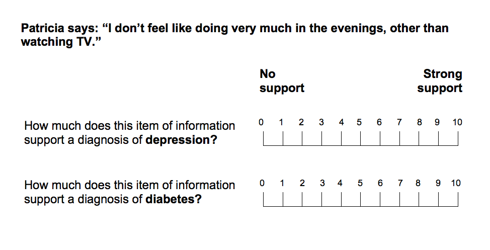
| Figure 1: Scales used to collect ratings of the diagnostic value of cues in the present studies. Participants were required to place one mark on each scale. The diagnosis evaluated first was counterbalanced across participants. |
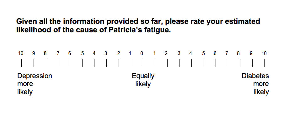
| Figure 2: Scale used to estimate diagnostic likelihood after 1) the steer and 2) the evaluation of each cue. The same scale was used in the study by Kostopoulou et al. (2012). |
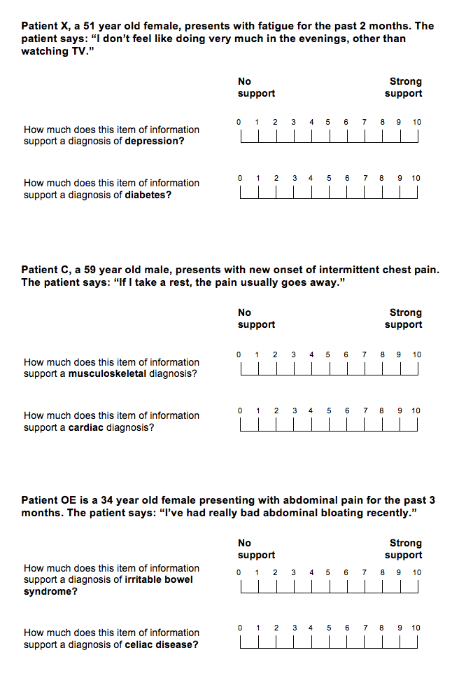
| Figure 3: Excerpt of materials seen by the control group. Participants were required to place one mark on each scale. The diagnosis evaluated first was counterbalanced across participants. |
Participants were required to respond to each item in turn. After they read the steer, they provided an estimate of diagnostic likelihood on a 21-point Visual Analogue Scale (VAS), anchored at “diagnosis A more likely” and “diagnosis B more likely”. Participants then assessed the diagnostic value of each neutral cue (and each conflicting cue, in scenario 3) for each of the two competing diagnoses. The manner in which they did so was the sole difference between the study by Kostopoulou et al. (2012) and the present one. In the 2012 study, participants rated the diagnostic value of each cue using a single 21-point VAS anchored at “favors diagnosis A” and “favors diagnosis B”. Hence, distortion was measured as the overall advantage afforded a leading diagnostic hypothesis. In the present study, participants rated the diagnostic value of each cue in relation to each diagnosis, using two 11-point VASs anchored at “no support” and “strong support” (Figure 1). Hence, distortion was measured separately for the leading and the trailing diagnostic hypotheses. Following each cue evaluation, participants updated their estimate of diagnostic likelihood, based on all information seen up to that point (Figure 2). They therefore provided three estimates in response to each cue (Figures 1 & 2).
Physicians in the control group evaluated the same cues as the experimental group. They used the same 11-point VASs (Figure 3) and therefore provided two ratings per cue. However, the control group did not have the opportunity to develop a leading diagnosis that could bias their cue evaluations (Russo et al., 1998; Kostopoulou et al., 2012). This was achieved in a number of ways:
1) All cues from the three scenarios were collected and scrambled, i.e., presented in a random order, different for each physician.
2) Each cue pertained to a new patient, introduced by a unique letter rather than a name (e.g., Patient A, Patient G), a health complaint (fatigue, dyspnea or chest pain) and minimal demographic information (sex and age).
3) Patient age was varied by a maximum of 4 years above or below the age specified in the corresponding scenario, to prevent participants from linking patients with the same health complaint and building a coherent representation. An experienced family physician and study co-author deemed that “…such small variations in age were not clinically significant” (Kostopoulou et al., 2012, p. 834).
4) Three decoy cues pertaining to entirely different pairs of diagnoses were included.
5) Participants were never asked to provide estimates of diagnostic likelihood.
2.2.4 Measuring of distortion
We measured distortion in two ways: the traditional way that averages cue ratings given by the control group to produce a point estimate of the “unbiased” rating per cue (“mean-based” method, DeKay et al., 2011), and a new way that takes into account the variation in control cue ratings.
2.2.5 The traditional way of measuring distortion
In most studies of distortion where participants use a single scale to rate the cues, distortion of a cue is calculated as the difference between an experimental participant’s cue rating and the mean cue rating by the control group. This difference is then signed as positive or negative depending on which option was leading just before the experimental participant rated the cue (“leader-signed” distortion, Russo et al., 1998).
In our study, physicians in both the experimental and control groups gave two ratings per cue, one in relation to diagnosis A and another in relation to diagnosis B. For each cue, we averaged the ratings of the control group in relation to each competing diagnosis, producing two mean control ratings per cue.
Each physician in the experimental group received two distortion scores per cue: one score in relation to the diagnosis that was leading just before the cue was evaluated and another score in relation to the diagnosis that was trailing just before the cue was evaluated. The diagnoses that were leading and trailing at any given time were identified from the physician’s most recent estimate of diagnostic likelihood (Figure 2).
To calculate distortion in relation to the leading diagnosis, we computed the difference between 1) a physician’s rating of a cue in relation to the leading diagnosis and 2) the mean control rating of the same cue in relation to the same diagnosis. A positive score indicated that the diagnostic value of information was overestimated to strengthen the leading diagnosis (“proleader distortion”, Blanchard et al., 2014; DeKay et al., 2014).
To calculate distortion in relation to the trailing diagnosis, we computed the difference between 1) a participant’s rating of a cue in relation to the trailing diagnosis and 2) the mean control rating of the same cue in relation to the same diagnosis. We then reversed the sign of the resulting difference, so that a positive score indicated that the diagnostic value of information was distorted to weaken the trailing diagnosis (“antitrailer distortion”, Blanchard et al., 2014; DeKay et al., 2014). Thus, positive distortion scores always indicated distortion in the predicted direction: strengthening the leading diagnosis and weakening the trailing diagnosis.
Table 1: Mean-based distortion in relation to the leading and trailing diagnoses in Study 1.
Mean (SD) Length 95% CI t (df), p Effect size (d) Distortion in relation to the leading diagnosis 0.20 (1.31) 0.54 [−0.07, 0.47] 1.50 (95), 0.14 0.15 (small) Distortion in relation to the trailing diagnosis 0.89 (1.22) 0.50 [0.64,1.14] 7.17 (95), <0.01 0.73 (med-large)
A new way of measuring distortion.
Mean-based distortion does not take into account the error of estimating the mean of the control group. If measured against an inflated mean control rating, proleader distortion would be underestimated and antitrailer distortion overestimated. Similarly, if measured against a diminished mean control rating, proleader distortion would be overestimated and antitrailer distortion underestimated.
To measure distortion in a way that accounts for the variance in the control cue ratings, we ran two 2-level mixed effects models: one to measure distortion in relation to the leading diagnosis and another to measure distortion in relation to the trailing diagnosis. We regressed the raw cue ratings on the study group (experimental vs. control), so that ratings cast under experimental conditions would be compared with ratings cast under control conditions, separately when a diagnosis was leading and when a diagnosis was trailing.
2.2.6 Sample size
In a linear regression of distortion on the estimated likelihood of a leading diagnosis, Kostopoulou et al. (2012) found that a 1-unit increase in diagnostic likelihood was associated with a 0.3-unit increase in physicians’ distortion on the next cue (slope = 0.3, p < 0.01). We estimated that to detect a similar association between diagnostic likelihood and distortion (the sum of proleader and antitrailer), with power of 0.8 and α = 0.05, we would need at least 71 participants in the experimental group. Likewise, the size of our control group was based on that of Kostopoulou et al. (2012) (n = 36).
2.3 Results
Of the 197 physicians e-mailed, 95 participated (48%). We recruited 44 additional participants at conferences, resulting in a final sample of 139 physicians: 50% female, 9% residents in family medicine, 28 to 64 years of age (M = 39.3, SD = 8.9, median = 36.0), with 0 to 36 years in family medicine (M = 10.1, SD = 9.5, median = 6.0). Demographics were comparable across the experimental (n = 96) and control (n = 43) groups.
2.3.1 Distortion in relation to the leading and trailing diagnoses
The traditional way of measuring distortion.
We averaged distortion in relation to the leading diagnoses across cues, per physician. We did the same for distortion in relation to the trailing diagnoses. One-sample t tests revealed that mean distortion in relation to the leading diagnoses was not significantly different from 0, while mean distortion in relation to the trailing diagnoses occupied almost one unit of the cue evaluation scale (Table 1). Paired-samples t tests revealed no reliable differences in the distortion of neutral vs. diagnostic cues (mean difference for distortion in relation to the leading diagnoses = 0.32 [−0.04, 0.68], t(95) = 1.76, p = 0.08, d = 0.18; mean difference for distortion in relation to the trailing diagnoses = 0.07 [−0.27, 0.41], t(95) = 0.38, p = 0.70, d = 0.04).
A new way of measuring distortion.
Variation in control cue ratings was substantial (mean SD = 2.07). Distortion in relation to leading diagnoses was not significant in the regression model: slope = 0.22 [−0.23, 0.66], p = 0.33. In contrast, the model that measured distortion in relation to trailing diagnoses found substantial antitrailer distortion: slope = −1.11 [−1.52, −0.70], p < 0.01. Thus, the new method of measuring distortion confirmed the findings of the traditional way of measuring distortion.1,2
Individual differences.
The two modes of distortion, each averaged per physician, were reliably different from one another (mean difference = 0.69 [0.23,1.15], t (95) = 3.01, p < 0.01, d = 0.31). We explored this further using paired-samples t tests per physician. We identified 17 physicians who displayed reliably more proleader than antitrailer distortion, and 31 physicians who displayed the opposite tendency. The remaining 48 physicians (50% of the sample) did not exhibit significant differences between the two modes of distortion.
To explore whether the tendency toward proleader vs. antitrailer distortion was consistent across scenarios, we calculated each physician’s mean proleader distortion and mean antitrailer distortion per scenario (excluding conflicting cues in the third scenario), and subtracted antitrailer from proleader distortion. A positive score for a scenario would indicate more proleader than antitrailer distortion, while a negative score would indicate the opposite. Cronbach’s α for the three scores was 0.79, suggesting that the tendency for proleader vs. antitrailer distortion was consistent for a given physician across scenarios.
Table 2: Diagnostic commitment in Study 1.
Chest Pain Dyspnea Fatigue Same side of diagnostic VAS at the start and at the end (i.e. after the neutral cues were evaluated) 92%* 71%* 79%* Same side of diagnostic VAS throughout (from the start until all neutral cues were evaluated) 80% 62% 62% * Fisher’s Exact p < 0.01
2.3.2 Distortion and diagnostic likelihood
We used a 2-level linear regression model with random intercept to investigate whether the estimated likelihood of the leading diagnosis accounted for the distortion on the next cue (DeKay et al., 2009; Kostopoulou et al., 2012). Separate models were created for each mode of distortion. The models used the distortion scores per cue, pairing each with the immediately preceding estimate of diagnostic likelihood. In both models, estimated diagnostic likelihood accounted for distortion on the next cue: slope = 0.14 [0.09, 0.19], p < 0.01 for distortion in relation to the leading diagnosis; slope = 0.09 [0.04, 0.13], p < 0.01 for distortion in relation to the trailing diagnosis.
We investigated whether each mode of distortion influenced the final diagnostic estimates in each scenario, after all the neutral cues had been rated and before any conflicting cues were seen in the third scenario (for comparability across scenarios). Table 2 shows the proportion of physicians who started and finished on the same side of the diagnostic likelihood VAS. It also shows the proportion of physicians who remained on the same side of the diagnostic likelihood VAS throughout a scenario. We excluded participants whose rating on the diagnostic likelihood scale was 0 (i.e., equal likelihood), either at the start or after the neutral cues were seen (n = 11 for chest pain, n = 19 for dyspnea, n = 15 for fatigue).
To explore the influence of each mode of distortion on final diagnostic estimates (i.e., estimates after all the neutral cues were seen and evaluated), we conducted a four-step analysis (DeKay et al., 2014).
Table 3: Associations with final diagnostic likelihood in Study 1.
Chest Pain Dyspnea Fatigue Initial diagnostic Beta = 0.57 Beta = 0.50 Beta = 0.47 likelihood B = 0.49 [0.37, 0.61] B = 0.32 [0.21, 0.42] B = 0.38 [0.25, 0.50] p < 0.01 p < 0.01 p < 0.01 Proleader distortion Beta = 0.16 Beta = 0.25 Beta = 0.27 B = 0.52 [0.20, 0.84] B = 0.68 [0.25, 1.11] B = 0.73 [0.31, 1.16] p < 0.01 p < 0.01 p < 0.01 Antitrailer distortion Beta = 0.37 Beta = 0.30 Beta = 0.35 B = 0.99 [0.62, 1.36] B = 0.71 [0.29, 1.14] B = 1.17 [0.67, 1.66] p < 0.01 p < 0.01 p < 0.01 Variance explained: 77% 46% 54% Total F (3, 91) = 105.94 F (3, 90) = 26.97 F (3, 91) = 37.06 p < 0.01 p < 0.01 p < 0.01 Variance explained: 8% 9% 13% Distortion F change (2, 91) = 16.50 F change (2, 90) = 8.00 F change (2, 91) = 13.52 p < 0.01 p < 0.01 p < 0.01 Note: Participants who did not develop a leading diagnosis in a given scenario were excluded from the analysis (n = 1 for chest pain, n = 2 for dyspnea, n = 1 for fatigue). Conflicting cues in the third scenario were excluded from the calculations. Variance explained Total expresses, as a percentage, the Adjusted R Square statistic for the full model. Variance explained Distortion expresses, as a percentage, the R Square Change statistic for the distortion component of the model.
1) We averaged per physician:
a. distortion in relation to Diagnosis 1 (D1) when it was leading,b. distortion in relation to D1 when it was trailing,
c. distortion in relation to Diagnosis 2 (D2) when it was leading, and
distortion in relation to D2 when it was trailing.
2) We reversed the signs for b and c, so that higher scores always favored D1.
3) We took the average of a and c (distortion in relation to leading diagnoses) and the average of b and d (distortion in relation to trailing diagnoses).
4) We used hierarchical linear regression to assess the relationship of these two averages with the final diagnostic likelihood (−10 = “D2 more likely”, 0 = “equally likely”, 10 = “D1 more likely”). We controlled for the diagnostic steer (counterbalanced across participants) as follows: initial diagnostic likelihood was the sole predictor in the first run of the model (block 1) and the two modes of distortion were added together subsequently (block 2).
Finally, we compared the coefficient for proleader with that for antitrailer distortion in each scenario, to determine any differences in their magnitude.
Our findings, presented in Table 3, were consistent across scenarios. The initial estimate of D1 likelihood was the strongest determinant of the final estimate of D1 likelihood. However, distortion to favor D1 made a small, independent contribution, with significant input from both proleader and antitrailer distortion. In two scenarios, dyspnea and fatigue, the two modes of distortion had roughly equal influence upon final judgments: F (1, 90) = 0.02, p = 0.88 for dyspnea; F (1, 91) = 2.44, p = 0.12 for fatigue. The influence of proleader distortion was significantly weaker than that of antitrailer distortion in the chest pain scenario: F (1, 91) = 4.74, p = 0.03.
2.3.3 Final diagnosis in the third scenario
At the start of the third scenario, the steer was successful in installing the intended leading diagnosis in 81 of the 96 physicians (84%); eight physicians considered the competing diagnosis more likely (8%), while the remaining seven physicians (7%) considered the two competing diagnoses equally likely (0-midpoint of the scale). At the end of the third scenario, after physicians had evaluated the three cues that opposed the initial steer, 32 considered the steer as more likely (33%), 52 physicians considered the competing diagnosis more likely (54%), and the remaining 12 considered the two diagnoses equally likely (13%).
3 Discussion
We measured physicians’ distortion of information in relation to a leading and a trailing diagnosis against the mean ratings of a separate control group. We also measured distortion using multilevel linear regression that bypassed the need to use mean control ratings as the baseline. The two ways of measuring distortion produced consistent findings. On average, we found minimal distortion to strengthen a leading diagnosis (proleader) but considerable distortion to weaken a competing, trailing diagnosis (antitrailer). However, analysis of proleader and antitrailer distortion per physician suggested individual differences, with a minority of physicians displaying predominantly proleader distortion. The higher the estimated likelihood of a leading diagnosis, the larger was each mode of distortion on the next cue. Increases in both modes of distortion were associated with increased final estimates of diagnostic likelihood. At the end of the third scenario, after physicians evaluated cues that conflicted with the initial steer, only about a third of the sample ended up considering the steered diagnosis more likely.
4 Study 2
4.1 Introduction
We expect that physicians’ cue ratings are informed by their unique constellation of medical knowledge and experiences. Therefore, variance resulting from individual differences in prior knowledge could be wrongfully attributed to distortion. The most valid estimate of distortion in medical diagnosis might thus be a “personalized” one (DeKay et al., 2011), where each participant’s distortion is measured relative to his/her own baseline ratings of cues.
DeKay and colleagues (2011, 2014) compared the personalized and mean-based measures of distortion directly. The personalized method did not provide a superior estimate: in fact, it was less precise than the mean-based one (DeKay et al., 2011). However, prior knowledge (or preference) was unlikely to influence cue evaluation in the study of DeKay et al. (2011), where undergraduates evaluated hypothetical gambles with which they had little or no experience. In DeKay et al.’s (2014) study, individual differences in preference for apartment features were clearly present, but the personalized and mean-based distortion measures still performed very similarly. Study 2 of the current article compared the personalized and mean-based estimates of distortion among physicians, whose prior knowledge and experience were relevant to the task at hand.
Study 1 revealed individual differences in the mode of distortion displayed. On average, physicians displayed predominantly antitrailer distortion, but a minority displayed predominantly proleader distortion. The dominant mode of distortion was consistent across scenarios. Study 2 tested two potential correlates of proleader and antitrailer distortion: the Personal Need for Structure (PNS) and the Personal Fear of Invalidity (PFI) (Thompson, Naccarato, Parker & Moskowitz, 2001). The PNS captures “…the need to create and maintain simple structures” (Neuberg, Judice & West, 1997, p. 1396; Neuberg & Newsom, 1993). Individuals with high PNS tend to assimilate incoming information to preexisting or emerging judgments. Therefore, we expected these persons to display greater distortion. The PFI measures the “…fear of making judgmental errors” (Neuberg et al., 1997, p. 1404). Individuals with high PFI tend to display ambivalent attitudes and indecisiveness (Neuberg et al., 1997; Thompson et al., 2001). Therefore, we expected them to provide lower estimates of diagnostic likelihood, which would in turn reduce the magnitude of distortion. Both scales have been shown to be valid and reasonably reliable (Thompson et al., 2001).
Previous attempts to identify personality variables that moderate distortion have generally proven fruitless. Russo et al. (1998) found no relationship between distortion and the Preference for Consistency (Cialdini, Trost & Newsom, 1995) or the Myers-Briggs dimension of judgment, while Meloy (2000) found distortion to be unrelated to the Need to Evaluate (Jarvis & Petty, 1996), the Need for Cognitive Closure (Kruglanski, Webster & Klem, 1993; Webster & Kruglanski, 1994; Kruglanski & Webster, 1996) and the PNS. However, these studies measured distortion as the total advantage afforded a leading alternative. Study 2 measured distortion in relation to competing diagnoses separately. It was therefore the first to explore whether personality variables might moderate mode of distortion (proleader and antitrailer) rather than total distortion.
4.2 Aims
- To compare the mean-based and personalized estimates of distortion, in participants with task-related prior knowledge.
- To explore potential sources of individual differences in the mode and magnitude of distortion, specifically, the Personal Need for Structure and Personal Fear of Invalidity.
Methods
4.2.1 Participant recruitment
We invited by e-mail UK family physicians and residents who had taken part in previous studies by the second author. Each participant received a £35 Amazon voucher as a token of appreciation. The voucher was of greater value than in Study 1, as participants were required to participate on two separate occasions and complete two additional questionnaires (PNS and PFI). We did not recruit physicians who had taken part in Study 1.
4.2.2 Materials and procedure
Only two changes were made to the materials and procedure of Study 1. Firstly, the study followed a within-participant design. Each participant completed both study conditions (experimental and control), in a counterbalanced order and with an interval of one month between conditions. The one-month interval was intended to remove potential carry-over effects (DeKay et al., 2011). Secondly, after a participant had completed both conditions, s/he was asked to complete two measures of individual differences: Neuberg and Newsom’s (1993) abbreviated version of the Personal Need for Structure scale (PNS, Thompson et al., 2001) and the Personal Fear of Invalidity scale (PFI, Thompson et al., 2001). Participants indicated their agreement with each of the 11 items of the PNS scale (e.g., I don’t like situations that are uncertain) and each of the 14 items of the PFI scale (e.g., I tend to struggle with most decisions). Agreement was rated on a six-point scale (1 = “strongly disagree” to 6 = “strongly agree”). The order in which the PFI and PNS scales were completed was counterbalanced across participants.
4.2.3 Calculation of distortion
The two modes of distortion (in relation to the leading and the trailing diagnoses) were calculated relative to the participant’s own ratings provided under control conditions on a separate occasion (“personalized distortion”). In an attempt to replicate the results of Study 1 with a new sample of physicians, we also measured distortion relative to the mean ratings that the whole Study 2 sample provided under control conditions (“mean-based distortion”).
Table 4: Personalized and mean-based estimates of proleader and antitrailer distortion in Study 2.
Mean (SD) Length 95% CI t (df), p Effect size (d) Proleader distortion (personalized) 0.09 (1.24) 0.52 [-0.17, 0.36] 0.69 (84), 0.49 0.07 (small) Antitrailer distortion (personalized) 0.82 (1.06) 0.45 [0.60, 1.05] 7.17 (84), <0.01 0.77 (med-large) Proleader distortion (mean-based) 0.19 (1.36) 0.58 [-0.10, 0.48] 1.30 (84), 0.20 0.14 (small) Antitrailer distortion (mean-based) 0.95 (1.24) 0.54 [0.68, 1.22] 7.03 (84), <0.01 0.77 (med-large)
4.3 Results
Of the 187 UK family physicians e-mailed, 91 participated (49%), a response rate almost identical to that in Study 1 (48%). Two were excluded from the analyses because they did not complete the second questionnaire. A further two were excluded because we subsequently discovered that they had participated in Study 1. Finally, two more were excluded because they got in touch to let us know that they had misunderstood the response scales. Our final sample consisted of 85 family physicians: 46% female, 1% residents, 25 to 63 years of age (M = 40.5, SD = 8.7, median = 37.0), with 0 to 35 years in family medicine (M = 11.3, SD = 9.1, median = 8.00). The sample was therefore comparable to that of Study 1, except that it contained a lower proportion of trainees (1% vs. 9%).
4.3.1 Distortion in relation to the leading and trailing diagnoses
The two modes of personalized distortion (personalized: calculated relative to each physician’s own control ratings) were each averaged across cues per physician. One-sample t tests revealed that personalized distortion in relation to the leading diagnoses was close to zero, while personalized distortion in relation to the trailing diagnoses was nearly one scale unit (Table 4). Personalized distortion did not differ between neutral and diagnostic cues (mean difference for proleader distortion = 0.31 [−0.03, 0.66], t (84) = 1.80, p = 0.08, d = 0.19; mean difference for antitrailer distortion = 0.10 [−0.29, 0.48], t (84) = 0.50, p = 0.62, d = 0.06).
The two modes of mean-based distortion (mean-based: calculated relative to the mean ratings of the Study 2 sample cast under control conditions) were each averaged across cues per physician. As in Study 1, one-sample t tests revealed that mean-based distortion in relation to the leading diagnoses approached zero, while mean-based distortion relation to the trailing diagnoses approached one unit on the cue evaluation scale (Table 4). As in Study 1, mean-based distortion did not differ between neutral and diagnostic cues (mean difference for proleader distortion = 0.29 [−0.08, 0.65], t (84) = 1.56, p = 0.12, d = 0.17; mean difference for antitrailer distortion = 0.11 [−0.26, 0.47], t (84) = 0.58, p = 0.57, d = 0.06). Thus, Study 2 replicated the findings of Study 1 in terms of mean-based distortion in relation to leading and trailing alternatives. Furthermore, the two different methods of measuring distortion (mean-based and personalized) produced very similar estimates of distortion magnitude and variance (Table 4).3
We compared the mean-based and personalized distortion estimates formally, using two paired-samples t tests, one per mode of distortion. Each t test compared the mean-based and personalized estimates of distortion for each physician. We found no statistical differences between the mean-based and personalized estimates for either mode of distortion (mean difference for proleader distortion = 0.10 [−0.17, 0.37], t (84) = 0.73, p = 0.47, d = 0.08; mean difference for antitrailer distortion = 0.12 [−0.12, 0.37], t (84) = 0.99, p = 0.33, d = 0.10).
As in Study 1, the two distortion modes were reliably different from each other, whether measured using the mean-based method (mean difference = 0.76 [0.26, 1.25], paired-samples t (84) = 3.03, p < 0.01, d = 0.33) or the personalized method (mean difference = 0.73 [0.31, 1.16], paired samples t (84) = 3.42, p < 0.01, d = 0.37). With the mean-based method, we identified 18 physicians (21%) who exhibited predominantly proleader distortion (18% in Study 1) and 30 physicians (35%) exhibiting predominantly antitrailer distortion (32% in Study 1). With the personalized method, we identified fewer physicians in each group: 9 physicians (11%) exhibited predominantly proleader distortion and 23 physicians (27%) exhibited predominantly antitrailer distortion. As in Study 1, the dominant mode of distortion was consistent across scenarios: Cronbach’s α = 0.81 for mean-based estimates (Cronbach’s α = 0.79 in Study 1), and Cronbach’s α = 0.67 for personalized estimates.
Table 5: Diagnostic commitment in Study 2.
Chest Pain Dyspnea Fatigue Same side of diagnostic VAS and at the end (i.e. after the neutral cues were evaluated) 87%* 76%* 83%* Same side of diagnostic VAS throughout (from the start until all neutral cues were evaluated) 81% 66% 70% * Fisher’s Exact p < 0.01.
4.3.2 Distortion and diagnostic likelihood
As in Study 1, the estimated likelihood of the diagnosis that was leading at any one time was significantly and positively associated with both modes of personalized distortion on the next cue: slope = 0.14 [0.08, 0.20], p < 0.01 for proleader, and slope = 0.10 [0.05, 0.16], p < 0.01 for antitrailer distortion. Almost identical slopes were obtained for mean-based distortion: slope = 0.14 [0.08, 0.20], p < 0.01 for proleader, and slope = 0.10 [0.04, 0.15], p < 0.01 for antitrailer distortion.
Table 5 shows the proportion of physicians who started and finished on the same side of the diagnostic likelihood VAS. It also shows the proportion of physicians who remained on the same side of the diagnostic likelihood VAS throughout a scenario.
We excluded participants whose initial and/or final rating on the diagnostic likelihood scale was 0 (i.e., equal likelihood) (n = 11 for chest pain, n = 18 for dyspnea, n = 19 for fatigue).
As in Study 1, we used hierarchical linear regression to assess the influence of the two modes of distortion on final estimates of diagnostic likelihood (after all neutral cues but before the conflicting cues in the third scenario), controlling for initial estimates. Separate models were created for personalized and mean-based distortion. Conflicting cues in the third scenario were excluded from the calculations. The results are reported in Table 6.
By and large, the personalized and mean-based models resemble those of Study 1: initial diagnostic likelihood had the strongest influence on final diagnostic likelihood, with distortion making a smaller, independent contribution. In two scenarios, dyspnea and fatigue, both modes of distortion were associated with final likelihood estimates, with roughly equal contributions thereto: personalized F (1, 80) = 2.20, p = 0.14, and mean-based F (1, 80) = 0.00, p = 0.94 for dyspnea; personalized F (1, 80) = 1.78, p = 0.19, and mean-based F (1, 80) = 0.18, p = 0.67 for fatigue. No association was observed for proleader distortion in the chest pain scenario, where the contribution of antitrailer distortion was significantly greater: personalized F (1, 80) = 7.64, p < 0.01, and mean-based F (1, 80) = 11.45, p < 0.01.
Table 6: Associations with final diagnostic likelihood in Study 2.
Chest Pain Dyspnea Fatigue Personalized Initial diagnostic Beta = 0.59 Beta = 0.55 Beta = 0.52 likelihood B = 0.53 [0.36, 0.69] B = 0.39 [0.27, 0.50] B = 0.40 [0.29, 0.51] p < 0.01 p < 0.01 p < 0.01 Proleader distortion Beta = 0.00 Beta = 0.23 Beta = 0.29 B = 0.00 [-0.46, 0.46] B = 0.67 [0.20, 1.14] B = 1.02 [0.52, 1.53] p > 0.99 p < 0.01 p < 0.01 Antitrailer distortion Beta = 0.29 Beta = 0.36 Beta = 0.35 B = 0.83 [0.30, 1.37] B = 1.07 [0.56, 1.59] B = 1.53 [0.90, 2.16] p < 0.01 p < 0.01 p < 0.01 Variance explained: 63% 56% 59% Total F (3, 80) = 48.96 F(3, 80) = 35.50 F (3, 80) = 41.54 p < 0.01 p < 0.01 p < 0.01 Variance explained: 5% 10% 17% Distortion F change (2, 80) = 5.20 F change (2, 80) = 9.33 F change (2, 80) = 17.75 p < 0.01 p < 0.01 p < 0.01 Mean-based Initial diagnostic Beta = 0.46 Beta = 0.54 Beta = 0.46 likelihood B = 0.41 [0.26, 0.56] B = 0.38 [0.27, 0.49] B = 0.35 [0.24, 0.46] p < 0.01 p < 0.01 p < 0.01 Proleader distortion Beta = 0.09 Beta = 0.34 Beta = 0.42 B = 0.31 [−0.13, 0.74] B = 1.00 [0.52, 1.48] B = 1.28 [0.86, 1.69] p = 0.17 p < 0.01 p < 0.01 Antitrailer distortion Beta = 0.44 Beta = 0.37 Beta = 0.34 B = 1.30 [0.82, 1.78] B = 0.99 [0.52, 1.46] B = 1.16 [0.69, 1.62] p < 0.01 p < 0.01 p < 0.01 Variance explained: 70% 58% 65% Total F (3, 80) = 64.43 F (3, 80) = 38.63 F (3, 80) = 51.78 p < 0.01 p < 0.01 p < 0.01 Variance explained: 11% 12% 23% Distortion F change (2, 80) = 14.44 F change (2, 80) = 11.82 F change (2, 80) = 26.42 p < 0.01 p < 0.01 p < 0.01 Note: Participants who did not develop a leading diagnosis in a given scenario were excluded from the analysis (n = 1 for chest pain, n = 1 for dyspnea, n = 1 for fatigue). Variance explained Total expresses, as a percentage, the Adjusted R Square statistic for the full model. Variance explained Distortion expresses, as a percentage, the R Square Change statistic for the distortion component of the model. Shaded cells denote departures from the findings of Study 1.
4.3.3 Final diagnosis in the third scenario
At the start of the third scenario, the steer was successful in installing the intended leading diagnosis in 74 of the 85 physicians (87%); five physicians considered the competing diagnosis more likely (6%), while six physicians considered the two competing diagnoses equally likely (7%). At the end of the third scenario, after physicians had evaluated the three cues that opposed the initial steer, 30 considered the steer as more likely (35%); 46 considered the competing diagnosis as more likely (54%), and the remaining nine physicians considered the two diagnoses equally likely (11%).
4.3.4 Individual differences measures
Responses to items of the Personal Need for Structure scale (PNS) were summed per participant. The mean PNS score was 41.4 (SD = 8.4, range 21 to 61). PNS did not correlate with either mode of distortion, whether calculated using the personalized method (leader distortion r = 0.04, p = 0.74; trailer distortion r = -0.06, p = 0.59) or the mean-based method (leader distortion r = 0.08, p = 0.48; trailer distortion r = -0.11, p = 0.30).
Responses to items of the Personal Fear of Invalidity (PFI) measure were also summed per participant. The mean PFI score was 45.4 (SD = 9.0, range 24 to 69). We found no significant relationship between PFI scores and initial estimates of diagnostic likelihood (Pearson r = −0.06, p = 0.57). As such, we no longer expected PFI score to correlate with either mode of distortion: personalized proleader distortion r = −0.06 (p = 0.58), mean-based r = −0.02 (p = 0.88); personalized antitrailer distortion r = 0.06 (p = 0.62), mean-based r = −0.09 (p = 0.40).
4.4 Discussion
Study 2 replicated the findings of Study 1, using both a personalized and a mean-based method for calculating distortion. On average, physicians displayed minimal distortion to strengthen a leading diagnosis and substantial distortion to weaken a trailing diagnosis. Again, we found individual differences in the mode of distortion, with a minority of physicians displaying predominantly proleader distortion. As in Study 1, the higher the estimated likelihood of a leading diagnosis, the larger was each mode of distortion on the next cue. An increase in either mode of distortion to favor one diagnosis tended to increase final estimates of its likelihood. This association was consistent across all three scenarios for antitrailer but not for proleader distortion. As in Study 1, at the end of the third scenario, after physicians evaluated cues that conflicted with the initial steer, only about a third of the sample ended up considering the steered diagnosis more likely.
Despite the expected relevance of prior knowledge to the task at hand, the personalized method for measuring distortion was statistically equivalent to the mean-based method. Neither mode of distortion correlated with Personal Need for Structure or Personal Fear of Invalidity.
5 General Discussion
In two studies, using two different samples of family physicians and two different methods of measuring predecisional information distortion in medical diagnosis, we divided distortion to its potential constituent modes: strengthening a leading diagnostic hypothesis or weakening a competing, trailing hypothesis. On average, we found consistent evidence for distortion to weaken a trailing hypothesis but not to strengthen a leading hypothesis. Only a minority of physicians engaged predominantly in proleader distortion. Physicians’ tendency to engage in one or the other mode of distortion was consistent across clinical scenarios. We explored two potential sources of individual differences, namely, Personal Need for Structure and Personal Fear of Invalidity. Consistent with previous research (Russo et al., 1998; Meloy, 2000; Russo et al., 2000), personality measures were not related to distortion.
In both studies, proleader and antitrailer distortion had similar effects upon final diagnostic judgments: an increase in either mode of distortion to favor a diagnosis was associated with increased final estimates of its likelihood. The influence of proleader distortion seemed weaker and less consistent across scenarios than that of antitrailer distortion, though the difference was significant for only one scenario in one study. Nonetheless, to the extent that proleader distortion occurred, it displayed the expected relations with emerging and final estimates of diagnostic likelihood (DeKay et al., 2014).
Two other research groups, entirely independently and almost simultaneously with our studies, used similar methods to investigate the different modes of distortion among lay people choosing consumer goods. They found evidence for both proleader and antitrailer distortion, which were of similar magnitude (Blanchard et al., 2014; DeKay et al., 2014).
The inconsistency with our findings could suggest that the processes underlying information distortion are specific to the study population and task (DeKay et al., 2014). There are plausible reasons why physicians might distort information to weaken a trailing diagnostic alternative rather than strengthen a leading one. Firstly, physicians are trained to generate multiple diagnostic hypotheses (a set of “differentials”) for the presenting problem. Subsequent information search aims to narrow down the set by excluding hypotheses rather than simply confirming a leading hypothesis (Elstein, Shulman & Sprafka, 1978), though the extent to which physicians do this in practice may vary. If their approach is indeed to exclude rather than confirm, then distorting information to weaken a trailing hypothesis may be more beneficial than distorting information to strengthen a leading one. If antitrailer distortion is sufficient in helping physicians to exclude the competing diagnosis, then they may not need to engage in proleader distortion as well.
Meloy and Russo (2004) found that distortion (conceptualized and measured as a single process) increased when there was a match between decision strategy (select vs. reject alternatives) and valence of alternatives (positive vs. negative): it was greatest when participants were required to select one of two positive alternatives or reject one of two negative alternatives. Their findings demonstrate that decision strategy can affect the magnitude of distortion; therefore, it may also affect the mode of distortion. Further research could explore the possibility that physicians’ predominant diagnostic strategy is responsible for the predominant mode of distortion found in our studies.
Secondly, the consequences of a misdiagnosis can be severe, arguably more severe than the consequences of selecting an inferior consumer item. Physicians may thus be prudent in evaluating diagnostic hypotheses. In our studies, this may influence their cue ratings within the diagnostic task (experimental condition) and not their ratings of random and seemingly unrelated cues (control condition). A conservative approach to the diagnostic task would curtail proleader but not antitrailer distortion. Future work could explore whether physicians’ perceived risk, inherent in the diagnostic task, is responsible for the predominant mode of distortion found in our studies.
Our findings have implications for theories of cognitive consistency, which suggest that information is distorted to maximize consistency between previously observed evidence, hypotheses and newly arriving evidence. As both modes of distortion can work to increase consistency, these accounts would predict the occurrence of both. The present findings pose a challenge to these accounts, calling for more research into the factors that might encourage one mode of distortion over another.
We note a difference between our findings on the final diagnosis in the third scenario and those of Kostopoulou et al. (2012). Across both studies reported here, 34% of physicians considered the steer as the most likely diagnosis after they evaluated the conflicting cues, in contrast to 49% reported by Kostopoulou and colleagues. Furthermore, 12% of physicians across both our studies considered the two competing diagnoses equally likely at the end of the third scenario, in contrast to 6% of physicians in the 2012 study. In summary, more physicians changed their diagnosis, and more gave the “normative” response of equal likelihood—normative because the net information in the third scenario (comprising steer cues, neutral cues, and conflicting cues) favored neither diagnosis. As the only methodological difference between the 2012 study and our two studies consists of the different cue evaluation scales (comparative vs. separate), this seems the most likely source of the different findings: the separate scales may have forced physicians to recognize evidence-based support for the opposing diagnosis at the end of the scenario, making it hard to dismiss. Although it is tempting to suggest that the separate scales operated akin to a “consider-the-opposite” debiasing strategy (Larrick, 2004), most physicians did not become more accurate but simply demonstrated a recency effect: switching to the opposite side of the diagnostic scale was more common than judgments of equal likelihood, suggesting that physicians placed more weight on the final cues. Nevertheless, judgments of equal diagnostic likelihood were somewhat more common than in the 2012 study, providing some hope that forced consideration of two possible outcomes could improve physicians’ diagnostic judgments.
We employed and compared two different methods for measuring distortion in physicians’ diagnostic judgments: a traditional “mean-based” method (Study 1) and a “personalized” method that has rarely been used (Study 2). In agreement with previous research (DeKay et al., 2011, 2014), they returned comparable results. This lends no support to the hypothesis that a personalized approach would outperform a mean-based one, when prior knowledge and experience are relevant to the task at hand. The logistics of following up participants, in our case physicians, to obtain their responses on a second occasion, while ensuring a time interval that reduces the likelihood of carry-over effects, are hard to achieve. Therefore, the mean-based method that relies on a separate control group offers an easier and equally valid alternative. However, the mean-based method is based on averaging the cue ratings of the control group; this ignores the error around these ratings, which could result in erroneous estimates of distortion. To address this, we developed a new strategy for analyzing SEP data. We used multilevel regression to compare cue ratings cast under experimental vs. control conditions, thus taking into account the variation in control group ratings. This analysis returned results consistent with the mean-based approach. This analytical strategy could be used to supplement and validate mean-based findings in future studies.
References
Blanchard, S. J., Carlson, K. A., & Meloy, M. G. (2014). Biased predecisional processing of leading and nonleading alternatives. Psychological Science, 25(3), 812–816.
Brownstein, A. L. (2003). Biased predecision processing. Psychological Bulletin, 129(4), 545–568.
Carlson, K. A., Meloy, M. G., & Russo, J. E. (2006). Leader-driven primacy: Using attribute order to affect consumer choice. Journal of Consumer Research, 32(4), 513–518.
Cialdini, R. B., Trost, M. R., & Newsom, J. T. (1995). Preference for consistency - the development of a valid measure and the discovery of surprising behavioral implications. Journal of Personality and Social Psychology, 69(2), 318–328.
DeKay, M. L., Miller, S. A., Schley, D. R., & Erford, B. M. (2014). Proleader and antitrailer information distortion and their effects on choice and postchoice memory. Organizational Behavior and Human Decision Processes, 125(2), 134–150. http://dx.doi.org/http://dx.doi.org/10.1016/j.obhdp.2014.07.003.
DeKay, M. L., Patiño-Echeverri, D., & Fischbeck, P. S. (2009). Distortion of probability and outcome information in risky decisions. Organizational Behavior and Human Decision Processes, 109(1), 79-92.
DeKay, M. L., Stone, E. R., & Miller, S. A. (2011). Leader-driven distortion of probability and payoff information affects choices between risky prospects. Journal of Behavioral Decision Making, 24(4), 394–411.
Elstein, A., Shulman, L., & Sprafka, S. (1978). Medical problem solving: An analysis of clinical reasoning. Cambridge, MA: Harvard University Press.
Glöckner, A., Betsch, T., & Schindler, N. (2010). Coherence shifts in probabilistic inference tasks. Journal of Behavioral Decision Making, 23(5), 439–462.
Holyoak, K. J., & Simon, D. (1999). Bidirectional reasoning in decision making by constraint satisfaction. Journal of Experimental Psychology: General, 128(1), 3–31.
Jarvis, W. B. G., & Petty, R. E. (1996). The need to evaluate. Journal of Personality and Social Psychology, 70(1), 172–194.
Kostopoulou, O., Mousoulis, C., & Delaney, B. C. (2009). Information search and information distortion in the diagnosis of an ambiguous presentation. Judgment and Decision Making, 4(5), 408–418.
Kostopoulou, O., Oudhoff, J., Nath, R., Delaney, B. C., Munro, C. W., Harries, C., & Holder, R. (2008). Predictors of diagnostic accuracy and safe management in difficult diagnostic problems in family medicine. Medical Decision Making, 28(5), 668–680.
Kostopoulou, O., Russo, J. E., Keenan, G., Delaney, B. C., & Douiri, A. (2012). Information Distortion in physicians’ diagnostic judgments. Medical Decision Making, 32(6), 831–839.
Kruglanski, A. W., & Webster, D. M. (1996). Motivated closing of the mind: “Seizing” and “freezing”. Psychological Review, 103(2), 263–283.
Kruglanski, A. W., Webster, D. M., & Klem, A. (1993). Motivated resistance and openness to persuasion in the presence or absence of prior information. Journal of Personality and Social Psychology, 65(5), 861–876.
Larrick, R. P. (2004). Debiasing. In D. J. Koehler & N. Harvey (Eds.), Blackwell handbook of judgment and decision making (pp. 316–337). Oxford: Blackwell.
Levy, A. G., & Hershey, J. C. (2008). Value-induced bias in medical decision making. Medical Decision Making, 28(2), 269–276.
Maloney, L. T., Martello, M. F. D., Sahm, C., & Spillmann, L. (2005). Past trials influence perception of ambiguous motion quartets through pattern completion. Proceedings of the National Academy of Sciences of the United States of America, 102(8), 3164–3169.
Meloy, M. G. (2000). Mood-driven distortion of product information. Journal of Consumer Research, 27(3), 345–359.
Meloy, M. G., & Russo, J. E. (2004). Binary choice under instructions to select versus reject. Organizational Behavior and Human Decision Processes, 93(2), 114–128.
Meloy, M. G., Russo, J. E., & Miller, G. C. (2006). Monetary incentives and mood. Journal of Marketing Research, 43(2), 267–275.
Miller, S. A., DeKay, M. L., Stone, E. R., & Sorenson, C. M. (2013). Assessing the sensitivity of information distortion to four potential influences in studies of risky choice. Judgment and Decision Making, 8(6), 662–677.
Montgomery, H., & Svenson, O. (1983). A think aloud study of dominance structuring in decision processes. In R. Tietz (Ed.), Aspiration levels in bargaining and economic decision making (pp. 383–399). Berlin, Germany: Springer-Verlag.
Neuberg, S. L., Judice, T. N., & West, S. G. (1997). What the need for closure scale measures and what it does not: Toward differentiating among related epistemic motives. Journal of Personality and Social Psychology, 72(6), 1396–1412.
Neuberg, S. L., & Newsom, J. T. (1993). Personal need for structure: Individual-differences in the desire for simple structure. Journal of Personality and Social Psychology, 65(1), 113–131.
Read, S. J., & Miller, L. C. (1993). Rapist or “regular guy”: Explanatory coherence in the construction of mental models of others. Personality and Social Psychology Bulletin, 19(5), 526–540.
Russo, J. E., Carlson, K. A., & Meloy, M. G. (2006). Choosing an inferior alternative. Psychological Science, 17(10), 899–904.
Russo, J. E., Carlson, K. A., Meloy, M. G., & Yong, K. (2008). The goal of consistency as a cause of information distortion. Journal of Experimental Psychology: General, 137(3), 456–470.
Russo, J. E., Medvec, V. H., & Meloy, M. G. (1996). The distortion of information during decisions. Organizational Behavior and Human Decision Processes, 66(1), 102–110.
Russo, J. E., Meloy, M. G., & Medvec, V. H. (1998). Predecisional distortion of product information. Journal of Marketing Research, 35(4), 438–452.
Russo, J. E., Meloy, M. G., & Wilks, T. J. (2000). Predecisional distortion of information by auditors and salespersons. Management Science, 46(1), 13–27.
Simon, D., Pham, L. B., Le, Q. A., & Holyoak, K. J. (2001). The emergence of coherence over the course of decision making. Journal of Experimental Psychology: Learning Memory and Cognition, 27(5), 1250–1260.
Simon, D., Snow, C. J., & Read, S. J. (2004). The redux of cognitive consistency theories: Evidence judgments by constraint satisfaction. Journal of Personality and Social Psychology, 86(6), 814–837.
Svenson, O., & Jakobsson, M. (2010). Creating coherence in real-life decision processes: Reasons, differentiation and consolidation. Scandinavian Journal of Psychology, 51(2), 93–102.
Thompson, M. M., Naccarato, M. E., Parker, K. C. H., & Moskowitz, G. B. (2001). The Personal Need for Structure and Personal Fear of Invalidity measures: Historical perspectives, current applications, and future directions. Paper presented at the Princeton Symposium on the Legacy and Future of Social Cognition Location, Princeton, NJ.
Tyszka, T. (1998). Two pairs of conflicting motives in decision making. Organizational Behavior and Human Decision Processes, 74(3), 189-211.
Tyszka, T., & Wielochowski, M. (1991). Must boxing verdicts be biased? Journal of Behavioral Decision Making, 4(4), 283–295.
Webster, D. M., & Kruglanski, A. W. (1994). Individual-differences in need for cognitive closure. Journal of Personality and Social Psychology, 67(6), 1049–1062.
- *
- Department of Primary Care & Public Health Sciences, Faculty of Life Sciences & Medicine, King’s College London.
- #
- Corresponding author: Department of Primary Care & Public Health Sciences, Faculty of Life Sciences & Medicine, King’s College London, 7th floor, Capital House , 42 Weston Street, London SE1 3QD, UK. Email: olga.kostopoulou@kcl.ac.uk.
- $
- Department of Psychology, University of Goettingen
- We would like to thank the Associate Editor, Michael DeKay, for his detailed comments and advice that helped to improve this manuscript. Thanks also to the Editor, Jonathan Baron, for pointing out the problem with the traditional way of calculating distortion.
All authors contributed to the design of the studies. Martine Nurek performed the data collection and analysis under the supervision of Olga Kostopoulou. Martine Nurek and Olga Kostopoulou drafted the manuscript, and York Hagmayer provided critical revision.
This research was supported by King’s ESRC Doctoral Training Centre studentship to Martine Nurek, and the NIHR Biomedical Research Centre at Guy’s and St Thomas’ NHS Foundation Trust and King’s College London.
Copyright: © 2014. The authors license this article under the terms of the Creative Commons Attribution 3.0 License.
- 1
- To compare the slopes for proleader and antitrailer distortion directly, we ran a single mixed effects model that compared raw cue ratings for the leading diagnosis, the trailing diagnosis, and the control group simultaneously. The slopes for proleader and antitrailer distortion were comparable to those of the separate models (slope for proleader distortion = 0.22 [−0.18, 0.62], p = 0.28; slope for antitrailer distortion = −1.11 [−1.51, −0.71], p < 0.01), and significantly different from one another (χ2 (1) = 5.06, p = 0.02). For the comparison of slopes we used their absolute values.
- 2
- Given the nearly significant difference in distortion between neutral and diagnostic cues in relation to the leading diagnosis, we also measured distortion on neutral cues only. Antitrailer distortion was significant: M = 0.90 [0.65, 1.16], t (95) = 6.95, p < 0.01, d = 0.70 in the traditional analysis; slope = −1.07 [−1.52, −0.63], p < 0.01 in the new analysis. Proleader distortion approached significance: M = 0.25 [−0.02, 0.51], t (95) = 1.86, p = 0.07, d = 0.19 in the traditional analysis; slope = 0.40 [−0.05, 0.86], p = 0.08 in the new analysis.
- 3
- When we reran the analyses for neutral cues only, antitrailer distortion was significant by both the personalized and mean-based methods of measurement (personalized M = 0.84 [0.60, 1.07], t (84) = 7.07, p < .01, d = 0.77; mean-based M = 0.95 [0.67, 1.23], t (84) = 6.80, p < 0.01, d = 0.74). Proleader distortion was not significant by either method of measurement (personalized M = 0.16 [−0.13, 0.44], t (84) = 1.10, p = 0.27, d = 0.12; mean-based M = 0.25 [−0.06, 0.55], t (84) = 1.62, p = 0.11, d = 0.18).
This document was translated from LATEX by HEVEA.