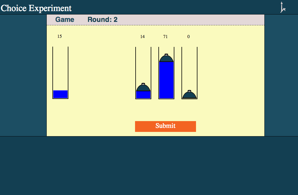
Figure 2: The investment screen (with three options).
Judgment and Decision Making, Vol. 9, No. 5, September 2014, pp. 373-386
Taking the sting out of choice: Diversification of investmentsJudith Avrahami* Yaakov Kareev# Einav Hart$ |
It is often the case that one can choose a mix of alternative options rather than have to select one option only. Such an opportunity to diversify may blunt the risk involved in all-or-none choice. Here we investigate repeated investment decisions in two-valued options that differ in their riskiness, looking for the effects of recent decisions and their outcomes on upcoming decisions. We compare these effects to those evident in all-or-none choice between the same risky options. The “state of the world”, namely, the likelihood of the high versus the low outcomes of the options, is manipulated. We find that aggregate allocation diverges from uniformity (i.e., from 1/n), and is sensitive to outcome probabilities, with the pattern of results indicating reactivity to the outcome of the previous decision. Round-to-round dynamics reveal that the outcome of the previous decision has an effect on the subsequent decision, on top of inertia; the aspects of the outcome that influence the next decision indicate an effect of a missed opportunity, if there was one, in the previous decision. Importantly, recent outcomes have a similar effect in diversification decisions and in all-or-none choice.
Keywords:diversification, choice, repeated decisions, missed
opportunities, bad luck.
Decisions often involve choosing one of several options—choosing among activities, among routes, among products, and so forth. But in many decision situations this is not necessarily the case: When deciding how to spend a free afternoon—doing sports or reading a book—one may choose to do a little of each; when deciding how to invest one’s savings one can choose to diversify: invest part of the savings in risky stocks and another part in safer bonds.
There is much theoretical work in economics about investing in risky assets, suggesting how a portfolio ought to be constructed to maximize profit, while taking risk attitudes into account (e.g., Markowitz, 1952; Shefrin & Statman, 2000). Such solutions are based on the expected values of the different assets, on the risk inherent in them, and on the weights of short-term and long-term gains. Behavioral research on decision making in general and on choice between risky options in particular has shown, however, that risks, gains and expected values are insufficient to explain people’s decisions. Consequently, there have been several attempts to incorporate affect—such as regret and disappointment—into theoretical models of investment strategies. For example, Muermann and Volkman (2006) proposed a dynamic portfolio choice model which, by incorporating anticipated regret and pride, can explain why investors sell winning stocks too early and hold on to losing stock for too long; Michenaud and Solnik (2008) incorporated anticipated regret into their financial decision-making model with the risk of regret added to traditional risk; and Gardner and Wuilloud (1995) found that institutional investors, who are judged over short periods, may greatly reduce the regret experienced over the strategy of investment while compromising the expected gains of a portfolio by only a little.
Experimental studies of the diversification of investments in risky assets focus mainly on the optimality of investors’ decisions. One line of research tested the effect of losses on investments (Thaler, Tversky, Kahneman, & Schwartz, 1997). Letting subjects diversify between assets differing in their risk—with the riskier asset having a higher expected value—Thaler et al. observed that optimality of investment was negatively related to the likelihood of a loss in the riskier, higher-level asset, and also negatively related to the frequency of portfolio evaluation.1 In another line of research the level of diversification was tested. Subjects’ investments were found to be more or less equally distributed between the available options (the 1/n rule, Benartzi & Thaler, 2001). This tendency often diverted investors from optimality (Kroll, Levy, & Rapoport, 1988; Rubinstein, 2002). Moreover, investors’ diversification behavior can be easily manipulated by changing the framing of the options or their categorization (Fox, Ratner, & Lieb, 2005; Read & Loewenstien, 1995; Sonnemann, Camerer, Fox, & Langer, 2013). Yet another related work tested subjects’ tendency to hedge their investment (e.g., Ben Zion, Erev, Haruvy, & Shavit, 2010). Offering a “hedge” option that provided the average of the payoffs of two negatively correlated options, and manipulating the level of feedback available, it was found that the safer, hedge, option was preferred only when feedback was limited to the option invested in—but not under complete feedback.
To the best of our knowledge, however, no experimental studies have focused on the interplay between a decision’s outcome and the next investment diversification. No study addressed the question of the influence of a decision’s unfavorable outcome—if there was any—in determining how the upcoming investment decisions would evolve.
This is not to say that the effect of experience has not been studied experimentally before. In fact, the effects of decisions’ outcomes on future behavior have been studied extensively, particularly in paradigms that involve uncertainty. The uncertainty stems either from not knowing the possible outcomes of gambles and/or the probabilities of the realization of these outcomes, or from not knowing what a counterpart would do. Various models of repeated decision behavior describe how different aspects of the experience, and the way memory operates in using that experience, determine behavior (e.g., Grosskopf, Erev, & Yechiam, 2006; Selten, Abbink, & Cox, 2005; Selten & Stoecker, 1986; Yechiam & Busemeyer, 2006). A central finding of these studies is that it is not only the actual but also the forgone payoff—the payoff that would have been received had one chosen differently—that influences choice. The operation of memory, namely, the sample of experience that is relevant for future decisions, and the relative weights of the actual and the forgone payoff are, however, still open questions (e.g., Erev & Barron, 2005; Selten & Chmura, 2008; Yechiam & Rakow, 2011).
We too have studied the effect of experience on the process of decision making, exploring how the outcome of the most recent decision influenced the next. This was studied for the case of choice between gambles (Avrahami & Kareev, 2011, Experiments 1 and 2; Hart, Kareev, & Avrahami, 2012) and for the case of strategic interactions (Avrahami & Kareev, 2011, Experiments 3 and 4; Kareev, Avrahami, & Fiedler, 2014). We have found that, independent of the task at hand, decisions were well explained by the outcome of the most recent decision: realizing, with hindsight, that the most recent decision was suboptimal, namely, that a different choice or a different action would have been more rewarding the decision maker was driven away from the previous decision to the one that turned out to have been better. The current study extends the previous ones into the case of diversification of investments. When decision makers can diversify between options rather than having to choose only one option or one action, the sting experienced from an unfavorable outcome may be diminished because the unfavorable outcome would involve only part of the investment. Therefore, reaction to outcomes may be subdued and long-term considerations prevail instead.
The main question in this paper is therefore whether a decision in which one could diversify would still be influenced by the outcome of the previous decision. If this is found to be the case, then the next question would be what in an outcome mattered: is the determining aspect the same for investment as for the all-or-none decisions formerly studied? Namely, is the decision driven by a comparison to what could have been earned had one acted differently? Or is the next investment decision driven by a comparison to what could have been earned had one been luckier? If, in contrast to previous findings for all-or-none decisions, diversification behavior is not affected by the experienced outcome of the previous decision, it may turn out that subjects adopt the 1/n strategy, or that they prefer a specific risk level, and invest accordingly.
In sum, our main objective was to find out if decisions regarding diversification of investments are at all sensitive to recent outcomes and, if they were, what aspect of the outcome has the strongest influence on the next decision. Behavior in such decisions was compared to that in all-or-none choice.
The current study includes a preliminary experiment with two available options—designed to test the paradigm of diversification initially—and a main experiment with three available options. In both experiments subjects were repeatedly presented with risky options (gambles), each having two possible values. On every round of the diversification paradigm subjects decided how to “invest” 100 points in those options, that is, they “chose a portfolio” for their endowment. After doing so, the realized values of all the options were revealed. The payoff in each round was the sum of the realized values of each option multiplied by the amount “invested” in that option. Data were compared to those observed in a choice paradigm in which the investment was confined to one option only.
Figure 1: The payoff structure of the different options (a) the two options in Experiment 1; (b) The three options in Experiment 2. (a)
Riskier gamble ⎧
⎪
⎪
⎪
⎨
⎪
⎪
⎪
⎩
High ⎛
⎝R ⎞
⎠
Low ⎛
⎝R ⎞
⎠
High ⎛
⎝S ⎞
⎠Low(S) ⎫
⎪
⎬
⎪
⎭
Safer gamble (b)
⎧
⎪
⎪
⎪
⎪
⎨
⎪
⎪
⎪
⎪
⎩
High ⎛
⎝R ⎞
⎠
Low ⎛
⎝R ⎞
⎠
High ⎛
⎝M ⎞
⎠Low(M) ⎫
⎪
⎪
⎬
⎪
⎪
⎭
High ⎛
⎝S ⎞
⎠Low(S) ⎫
⎪
⎬
⎪
⎭
The design of the experiments included two special features aimed at uncovering possible effects of the outcome on the next decision and a third feature aimed at increasing the comparability of the diversification and the choice paradigm. The first feature was the ranges of outcome-values of the options—which were different for the different options—such that the range of one was included in that of another. As a result, the option with the widest range was riskiest, and the option with the narrowest range was safest (see Figure 1). To eliminate issues of optimality we chose the options such that their expected values were (almost) the same. As explained below, this feature of the design allowed us to directly test which comparisons, if any, influenced behavior.
A second feature of the design was the overall “goodness” of the situation—the “state of the world”, as it were—operationalized through the likelihood of the high outcome-values of the options. This was above 50% in the “good world” and below 50% in the “bad world”. World goodness thus determined the expected value of all the options, which was higher in a good than in a bad world. As will be shown below, models based on reactivity to outcome predict an effect of world on the average investment in the various options—in spite of the similarity in expected value—with the reactivity to different aspects of the outcome predicted to have different effects. Obviously, the 1/n strategy does not.
A third feature of the experiment, designed to increase the comparability of the paradigms of investment and choice, was to allow investment to be continuous. Because in a choice paradigm subjects do not commit to the numeric proportions of choosing either option, we wanted to make sure that they also do not have to commit to exact numeric proportions in their investments. This was done to avoid the danger of attraction to certain numbers—like round numbers, or numbers with a specific relation between them. Therefore, instead of asking subjects to state, in numbers, how much they would like to invest in each option, we created an environment in which subjects transferred their endowment, realized as “fluid”, from a source container into “tubes” that represented the options. Fluid was transferred to and from the tubes by drawing the tubes’ lids up or down (see Appendix A).
The main question was whether and how aspects of an outcome of one investment decision influence the following one. Naturally, an important aspect of the outcome of a decision is the reward earned from the options. As has been noted above, however, this reward is likely to be considered in comparison to what could have been earned. It could be compared to what would have been earned had one invested differently. In that case, one may notice that one has missed an opportunity to earn more (henceforth referred to as “miss”). Earnings could be compared also to what one could have earned had one been luckier and the high rather than the low value(s) of options realized (henceforth referred to as “bad luck”).
With regard to the comparison of an outcome to what could have been earned had one invested differently (i.e., whether or not an opportunity was missed), it is important to note that, with the current design, payoff would always be different if one had invested differently. To illustrate, let us consider the case of two options (see Figure 1a). Each option can have one of two outcome values—a high value and a low value. With the range of outcomes of one option being wider than that of the second, the high value of the former is higher than both values of the latter and the low value of the former is lower than both values of the latter. Let us call the former option the “riskier” option (R) and the latter option the “safer” option (S). Whatever was invested in the R option would be regarded as a miss if this option came out low and whatever was invested in the S option would be regarded as a miss if the R option came out high. Thus, if what drives the next investment is reaction to the mere occurrence of a miss, it is always the outcome value of the R option that determines whether or not the investment was a miss, both with regard to investments in the R and in the S option. Thanks to this design, a regression analysis of investment in a round (with the previous outcome of both options as predictors) should display only an effect of the realized value of the R option if behavior reflects reaction to misses.
The value realized in an option could also be compared to the other possible value of the option invested in. If behavior were driven by an assessment of luck it would result in retraction from an option when its low value is realized. In that case, the outcome in both the R and the S options would have an effect on the next investment and a regression analysis should display both an effect of the realized value in R and an effect of the realized value in S.2
Another comparison that may be at work is the size—and not just the occurrence of—the difference between what was and what could have been earned had one invested differently. In other words, not merely whether or not investment turned out to be a miss, but also how much was missed that is, the sum of the missed earnings. In that case, an interaction between the outcome in R and the outcome in S is to be expected.
To summarize, an effect of the outcome in the S option (or an interaction between the two outcomes) would indicate that it is not merely the realization that the previous investment involved a miss that influences the next decision. It could be that reaction to bad luck played a role or that the magnitude of the miss involved in one’s investment played a role. To anticipate, no effect of the outcome of S or its interaction with the outcome of R was found. We therefore do not elaborate on all the alternative models that could explain an effect of the outcome of S.
So far we have discussed the case of two available options. Predictions are more complex for the case of three options, but they follow the same logic. Here too, if what drives the next investment is a reaction to the mere occurrence of a miss in the part of the investment that could have produced higher earnings, investment in R should be influenced only by the outcome in R, because a high value in R is the highest possible outcome and a low value in R is the lowest. Investment in the medium-risk option (M), however, would be influenced not only by the outcomes in R but also by the outcome in M. This is because although following a high in the R option should divert investments towards R and away from the other two, the target of what was invested in R following a low in that option depends on the realized value in the M option: if the M value is high—investment is expected to be shifted there—but if low, it would be shifted to the S option. This would also determine how investment in option S should be affected: Investment in the safest option S should be influenced by the outcomes in R and in M. And, because the outcome in M is relevant only when the low outcome in R occurs, an interaction between the outcomes of R and M is expected as well. No influence of the outcome in S is expected.3
Table 1: Outcomes that would drive the next investment in the different options
Miss Lack of luck Size of miss
As in the case of two options, if behavior were driven by an assessment of luck, the next investment in each of the three options would be influenced by the realized values of all three options—R, M, and S. If the size of the earnings missed is the driving force then all three outcomes together with the interaction between all of them (i.e., R*M*S) should be observed. Table 1 summarizes what aspects of an outcome should influence the next investment according to the various driving forces considered.
In deriving predictions for average investment across rounds we shall assume first that decision makers react fully to the occurrence of misses alone and change their investments (from round to round) accordingly, and then assume that they react fully to whether or not they have been unlucky, namely, to whether or not the actualized value of any option was low. If investment changed in reaction to the outcome (whether through reaction to misses or to bad luck), the aggregate investment in each option would reach equilibrium such that the probability that investing in an option was a miss (or unlucky) equals the probability that not investing in that option was a miss (or unlucky). This equilibrium is inspired by Selten’s Impulse Balance concept (Selten et al., 2005; Selten & Stoecker, 1986), which defines the resting point of the Learning Direction Theory.
Solving the relevant equations for the miss-based equilibrium (see Appendix B) shows again that investment in the R option should be related only to the likelihood of the high value in the R option. The effect in the rest of the options is, as before, different for the case of two and three options. In the case of two options, investment in the S option is simply the complement of investment in the R option and hence corresponds to the likelihood of the low value in the R option. In the case of three options the predictions for the M and S options depend, as before, on the outcome of both the R and the M options. The exact numeric predictions for the average investment, for the parameters used in each experiment, will be presented in the results sections of the experiments.
If decisions are driven by the luck regarding the outcome in an option, then the likelihood of investing in one option and being unlucky with it should be equal to the likelihood of investing in the other (in the case of two options) and being unlucky with it (see Appendix C). In the case of three options, it should be equal to half the likelihood of being unlucky with each of the other two options. Thus, the outcome value of all options must enter the equations.
Because the numeric predictions for average investment in the available options are based on the values of the options and their probabilities, the predictions differ for the different worlds. Importantly, the predictions for the difference between worlds are not the same for the two equilibria and are, in fact, in opposite directions. According to the miss-based equilibrium, the average investment in the riskiest option would be higher in a good than in a bad world because investment in the riskiest option is proportional to the likelihood of a high outcome value in that option. According to the luck-based equilibrium, in contrast, investment in the riskiest option would be lower in a good than in a bad world. To understand why this is so one should note that the likelihoods of both values in the less risky option(s) are more extreme than those in the R option (to counter the less extreme outcome values while keeping the expected value the same), and that investment is inversely related to the likelihood of getting the low outcome value (i.e., being unlucky).4 As a result, the likelihood of a low outcome value is higher in the riskiest than in the safer options in a good world; the opposite is true in a bad world.
An important aspect of the equilibria is that the state of the world enters the equations only through the likelihoods of occurrence of the various outcomes. Thus, the effect of world on aggregate investment/choice stems only from the statistical characteristics of the states; it is not based on different assumptions regarding reactivity to outcomes. Therefore, while predictions based on either reaction to miss or reaction to no luck imply an effect of world on aggregate behavior, neither type of reaction predicts an effect of world on the dynamics of behavior. Interactions of world with outcomes are expected for aggregate behavior but not for its behavior dynamics.
Yet another possible prediction concerning average investment is based on the assumption that small probabilities are underweighted.5 Given the design of the options, the rarest events are the low value of the S option in a good world and the high value of the S option in the bad world; these values are candidates for underweighting. If these were indeed underweighted then the S option would look better than the R option in a good world, and look worse than the R option in the bad world. This, in turn, should result in a pattern of results similar to that of the luck-based equilibrium: Investment in the R option lower in the good world than in the bad one.
As aforementioned, Experiment 1 was a preliminary experiment designed to test the diversification paradigm and provide an initial comparison to behavior in a choice paradigm from data collected for a different study (Hart et al., 2012).
On each of 80 rounds, subjects either divided 100 points between two options in the diversification paradigm, or chose one option in the choice paradigm. After pressing “continue” the realized values of the options and the subjects’ current earnings were presented. Subjects thus knew what they would have earned had they invested (chosen) differently. For each round, earnings were equal to a proportion of the realized values of the options, corresponding to the proportion invested in each (in the diversification paradigm) or the full value of the option chosen (in the choice paradigm).
The experiment was conducted individually. After reading the instructions, subjects in the diversification paradigm were presented with a screen depicting three tubes. One—the source tube—was full and the other two tubes—representing the options—were empty. The latter two tubes had lids that could be dragged up or down. Subjects were instructed to divide the liquid of the source tube between the two empty tubes as they saw fit, by dragging the respective lids. In the choice paradigm, subjects simply clicked on the option of their choice.
After using up all the fluid from the source tube (or choosing an option) subjects pressed “continue” and the realized values of the two options, together with the summarized payoff for that round, appeared on the screen. Following another press on the “continue” button a new round began.
The possible outcome values of the options were (9, 3) in the riskier (R) option and (7, 5) in the safer (S) option. The likelihoods of the higher outcomes in both options were high in the good world (.633 and .900 in the R and S options, respectively), and low (.367 and .100), in the bad world. Thus, in the good world R was (9, .633; 3) and S was (7, .900; 5); in the bad world R was (9, .367; 3) and S was (7, .100; 5).
Note that, as mentioned above, the probabilities are more extreme for the S than for the R option. The location of the R and S options was randomized across subjects. Unbeknownst to the subjects, world changed after 40 rounds. Order of worlds was counterbalanced with half of the subjects first facing a good world and the other half facing a bad world first.
Eighty acquaintances of the experimenter participated in the diversification experiment and the data of 34 students who participated in a previous, choice, study were used for comparison. These 34 subjects are a subset of the subjects in the Hart et al. (2012) study for whom parameters were closest to the current experiment.6 Subjects earned, on average, 20 New Israeli Shekels (NIS, with one NIS worth approximately 0.28 US dollars at the time of the study).
The design of the experiment (together with the old data) was a 2 (Paradigm: diversification vs. choice) X 2 (World: good vs. bad) with the first variable manipulated between subjects and the second manipulated within subjects.
The results section presents the average, aggregate, investment in the options and then the effects of outcome in a round on behavior in the next.
Looking for the signature of reactivity to outcome, which should manifest in an effect of world on average investment, we first compared how investment was split between the options in the two worlds. Investment in the R option was 55.2% (SD=14.4) in the good world and 49.1% (SD=14.6) in the bad. An analysis of variance on average investment, with world as a within-subjects variable, reveals that this difference is significant (F(1,79)=14.92, p<.001, η2 =.159). This sensitivity to the state of the world indicates that reaction to outcome was at work. The difference in average investment in the two worlds corresponds well to that in the choice data, where average investment was 53.2% in a good world and 48.4% in a bad. Thus, the direction of the difference, namely, a higher average investment in R in the good world, is in line with the miss-based predictions rather than with the luck-based (or with underweighting of small probabilities) predictions. At the same time, although the relation between investments in the two worlds is in line with the miss-based and not with the luck-based predictions, the averages are much less extreme than predicted. More specifically, according to miss-based predictions the values should have been 63.3% in a good and 36.7% in a bad world whereas according to luck-based predictions they should have been 21.4% in a good and 58.7% in a bad world.7 Order in which the worlds were experienced had no effect on investment or choice (F< 1).
The diversion from the miss-based predictions could be a result of a weak effect of reaction to being unlucky that was exceeded, and therefore masked, by the effect of the reaction to miss; it could be a result of only a weak effect of the magnitude of the miss; or an effect of inertia (e.g., Erev & Haruvy, 2005). A detailed analysis of the aspects of an outcome that influenced the next investment could reveal either or all of these effects. More specifically, if being unlucky with an outcome has an additional influence on behavior then an effect of the outcome value in S should be observed; if the magnitude of the miss has an influence then an interaction between the outcome values in R and in S is expected and if the shadow of past experience also influences decisions then an effect of the current choice—embodying reaction to previous experience—would be evident.
Table 2: Results of the regression analysis predicting the next investment in (or choice of) R by the current investment (or choice), the outcome values of R and S, and paradigm (choice vs. diversification) displaying coefficients (error terms) and significance levels.
factor nextR current_in_R 0.239 (0.036)*** outcomeR 0.038 (0.004)*** outcomeS −0.010 (0.005)* outRxoutS −0.0005 (0.002) Paradigm −0.185 (0.179) ParadigmxoutR 0.005 (0.028) ParadigmxoutS 0.055 (0.029) Paradigm·outRxoutS −0.004 (0.005) constant 0.486 (0.093)*** F(8,113) = 23.83; p < .001; R-squared = 0.123; Root-MSE = 0.382; N=8972, clusters = 114. * < 0.05; ** < 0.01; *** < 0.001
For the analysis of the aspects of a round’s outcome that might have influenced the next decision, we conducted a regression analysis with the various aspects as predictors. Given the similarity in the effect of world on the averages of investment and of choice, a single regression analysis was performed for both paradigms, using paradigm as an additional predictor. The variables characterizing a round were the realized value in the R option, the realized value in the S option and the current investment (in the R option). There were two reasons for including the current investment: to find out if behavior was subject to either regression-to-the-mean or to inertia—and if it was (to either), to see what effects of outcome remained. The results of the regression analysis—with the model’s variance clustered by subjects8—are presented in Table 2.
As is evident from Table 2, two variables were most strongly related to the next choice: the current choice and the outcome in the R option. Current choice had a strong positive effect indicating inertia, and the outcome in the R option, having a positive effect too, indicates that a high in R increased the next investment in (or the tendency to choose) R. An effect of the outcome in the S option—albeit weaker—was significant as well. This effect is not in line with the predictions based on miss alone, and can support predictions based on how unlucky one was with the outcome. The effect of the outcome in S is only partially compatible with predictions based on the magnitude of the miss because this would require also an interaction between the two outcome values.
There was no main effect of paradigm (diversification or choice), nor an interaction of paradigm and the realized value in R. That is, the outcome in R had a similar effect in both paradigms.
Although only a preliminary study, Experiment 1 already provides several indications regarding the questions of the study. First, an effect of outcomes was observed, which supported the assumption that investment decisions were influenced by reaction to the outcome of the previous decision. Second, and perhaps most interesting, we did not observe an effect of paradigm: apparently, the opportunity to diversify did not change the choices subjects made, nor the way subjects reacted to their experience. Third, a strong effect of inertia was observed, indicating that the shadow of the past was at work as well.
Table 3: Probability of the R option turning out higher than the S option in different sample sizes drawn randomly in the good world. Values in the bad world are the complements of these values. Compare these to 0.552 observed in the data.
Sample Size Probability of R better than S 1 0.633 2 0.447 3 0.534 4 0.542 5 0.480 6 0.528 7 0.518 8 0.495 9 0.521 10 0.509
It may be worth pausing here to try and unpack the effect of inertia and see how it may be related to past experience. Having already found that behavior was mainly driven by an ordinal comparison of the observed outcomes of the available options (rather than by the size of the difference or by comparison to the observed mean of each option), one could try to estimate the length of the “shadow” of past experience. To do that, one could calculate the likelihood of an option coming ahead for different sizes of samples of past experience and see which of them best fits the data.9 We calculated the likelihood of the R option turning out higher for a number of sample sizes. Table 3 presents these results for sample sizes of 1 to 10. As can be seen in the table, there are several sample sizes that could explain the exact ratio observed in the data, for example 3 and 4. One could also assume a mixture—different subjects using different sizes, or subjects using a variety of sizes—and get the proportions that fit the data. If, for example, one assumes that each subject chooses randomly, and with equal probability, samples of sizes between 1 and 9, or that an equal number of subjects use each sample size between 1 and 9 (Erev & Roth, 2014), one gets .522 in the good world—a good fit as well. Having noted that, we return to the main thrust of the paper.
The first experiment employed only two options, which allows for limited diversification. Experiment 2 amends this point, and was designed to increase the generality of the findings.
This experiment used the same two paradigms—diversification and choice—as Experiment 1, but differed from it in several respects. The two main differences were that (a) three options were available for investment or choice instead of two; (b) the possibility of losses was introduced, with all options having a negative as well as a positive outcome value. Other differences concerned the manipulation of world—which here was manipulated between subjects—and the ambience of the experiment—this experiment was run over the Internet at the subjects’ preferred time and location (rather than with an experimenter).
As in Experiment 1, both possible outcome values of a safer option were included in those of the riskier one: The possible outcome values of the options were (9, −3) in the riskiest (R) option, (8, −2) in the medium-risk (M) option, and (7, −1) in the safest (S) option. As in Experiment 1, worlds corresponded to the expected value of all options, which was operationalized through the probabilities of the higher outcome-values in the options. In the good world the likelihoods of a high value were .667, .710, and .750 (in the R, M, and S options, respectively), and in the bad world they were .333, .310, and .250, respectively. Thus, in the good world R was (9, .667; −3), M was (8, .710; −2), and S was (7, .750; −1); in the bad world R was (9, .333; −3), M was (8, .310; −2), and S was (7, .250; −1).
Here too, the locations of the R, M, and S options were randomized across subjects. World was manipulated between subjects. Note that in both worlds the expected value of the (M) option was slightly superior to the other two, which were identical in their expected value. The difference amounted to 0.1 of a point. This difference was introduced to see if the expected value of this option attracted a higher share of investments than that predicted by the two equilibria, which would indicate maximizing behavior rather than mere reactivity to outcomes.
Subjects performed 80 rounds in the faster, choice paradigm and 40 rounds in the diversification paradigm.
One hundred and twenty students participated in the experiment. Subjects were recruited to an experiment on the Internet by ads on campus or through Facebook. To guarantee that subjects were students even though the experiment was conducted over the Internet, they had to come and present their student identification in order to collect their remuneration. Subjects earned, on average, 18 NIS (one NIS about $0.28).
The design was similar to that of Experiment 1: 2 (paradigm, diversification or choice) X 2 (world, good or bad). Unlike in Experiment 1, here both independent variables were manipulated between subjects; the computer program randomly determined assignment to experimental group.
As in Experiment 1, we first calculated the average proportion of investment (or choice) in each option for each subject, separately for each paradigm and each world. We used an analysis of variance to compare these proportions in the riskiest and the safest options, as a within subjects variable, and with world and paradigm as between subjects variables. Time—first or second half of the rounds—was another within subjects variable. This analysis revealed a significant main effect of the options’ risk level, namely, a difference between the investment (and choice) rates in the two extreme options, with higher investment (or choice) in the R option (F(1,115)=10.42, p=.002, η2=.083).10 Importantly, there was a significant interaction between riskiness and world, with investments (or choice) in the riskiest option higher in the good than in the bad world (F(1,115)=9.66, p=.002, η2=.077). This result is in line with the miss-based predictions but not with the luck-based predictions. Paradigm had no main effect nor did it enter any of the interaction terms (all F’s<1); that is, there was no difference in choice patterns between the diversification and choice paradigms.The observed means—lumped over paradigm and time—and the predictions of miss- and luck-based equilibria, separately for the good and bad worlds, are presented in Table 4.
Table 4: Observed and predicted percentages of investment (or choice) in the three options, separately for the two states of the world. “Miss” represents the prediction of a miss-based model and “Luck” the prediction of a lack-of-luck model.
Bad world Good world Riskiest Observed 33.8 41.1 Miss 33.3 66.7 Luck 35.0 28.7 Medium Observed 31.8 35.2 Miss 20.7 23.6 Luck 33.9 33.0 Safest Observed 34.4 23.8 Miss 46.0 9.7 Luck 31.1 38.3
As is evident from comparing the two columns of Table 4, the ordinal relation of investment in (or choice of) the R versus the S options (i.e., R higher and S lower in the good than in the bad world) is in line with the miss-based predictions. At the same time, the actual averages are, as in Experiment 1, far less extreme than those predicted. Further, at least in a bad world, they are indistinguishable from uniformity. One possible explanation for this diversion from predictions could be a reasoned draw towards the more valuable M option, since investment in the M option always exceeded that predicted by the miss-based equilibrium. This account fails, however, in explaining why in a bad world the two extreme options (R and S) received the same share of investment.
There was a significant effect of time, expressed in a three-way interaction between time, the options’ risk level, and world (F(1,115)=4.69, p=.032, η2=.039): Over time, investment in (or choice of) the riskiest option became higher in the good world and lower in the bad, whereas investment in (or choice of) the safest option became lower in the good world and higher in the bad. These changes represent a shift, over time, towards the predictions of reactivity to miss.
To see what could bring about the pattern of results reported in Table 4 we now turn to behavior dynamics through a regression analysis of the effect of the outcome of a round on behavior in the next round.
We remind the reader that, although luck-based and magnitude-of-miss-based predictions involve the same outcome values to predict the next investment in (or choice of) all three options, this is not true for predictions based on miss alone. Unlike in the case of two options, in which whatever influences investment (or choice) in the R option influences—by definition—also investment (or choice) in the complementing S option, the predictions for the aspects that influence behavior in the case of three options are not the same for all three options. In the three options case, the predictions based on reaction to misses are as follows: the next investment in (or choice of) the R option ought to be influenced only by the realized value in the R option. In contrast, investment in (or choice of) the M and S options would be influenced by the realized value in the R option and the M option, as well as the interaction between them.
Table 5: Results of regression analyses with paradigm (choice vs. investment) separately for each option (R=riskiest, M=medium, S=safest). “Current” indicates the current investment/choice in the relevant option such that for the analysis of nextR current=investment in R and so forth. Presented are the coefficients (error terms) and significance levels.
factor nextR nextM nextS current 0.257 (0.041) *** 0.276 (0.046) *** 0.216 (0.051) *** outcomeR 7.651 (1.030) *** −3.600 (0.712) *** −4.036 (0.753) *** outcomeM −1.548 (0.822) 5.905 (0.965) *** −4.436 (0.795) *** outcomeS 0.606 (0.745) −1.965 (0.754) ** 1.239 (0.876) outR·outM −0.552 (0.714) −1.483 (0.566) ** 2.035 (0.611) ** outR·outS 0.710 (0.665) 0.233 (0.545) −0.935 (0.638) outM·outS 1.121 (0.719) −0.159 (0.564) −0.932 (0.685) outR·outM·outS 0.048 (0.671) −0.335 (0.521) 0.295 (0.588) Paradigm 0.974 (1.320) −1.060 (1.242) 0.083 (1.173) Paradigm·outR −1.765 (1.029) 1.020 (0.708) 0.749 (0.752) Paradigm·outM −0.367 (0.823) −0.648 (0.966) 1.008 (0.788) Paradigm·outS 0.330 (0.745) −0.306 (0.764) −0.046 (0.835) Paradigm·outR·outM 0.092 (0.717) 0.451 (0.585) −0.539 (0.628) Paradigm·outR·outS 0.408 (0.611) 0.164 (0.542) −0.620 (0.580) Paradigm·outM·outS 0.450 (0.673) 1.013 (0.691) −1.440 (0.650) * Paradigm·outR·outM·outS −0.327 (0.652) −0.157 (0.547) 0.485 (0.580) constant 28.294 (1.778) *** 24.348 (1.659) *** 22.181 (1.378) *** F(16, 119) = 7.32 F(16, 119) = 10.48 F(16, 119) = 7.09 p < .001 p < .001 p < .001 R-squared = 0.1023 R-squared = 0.1068 R-squared = 0.0804 Root MSE = 40.68 Root MSE = 39.00 Root MSE = 37.559 N=4613, clusters = 120. * < 0.05; ** < 0.01; *** < 0.001.
Therefore, a single regression analysis could not suffice for learning how investment (or choice) in each option was related to the aspects of the previous round. Instead, three regression analyses, separately for each of the three options, were conducted.11 The three outcome values (and their interactions) were used as predictors together with the current investment in (or choice of) an option. In addition, paradigm and its interactions with the other predictors were included in the analyses. The results of these regression analyses are presented in Table 5.
As in Experiment 1, there was a positive effect of the current investment or choice on that in the next, indicating inertia. There was, however practically no effect of paradigm (or its interactions with the outcomes) on behavior in the next round. This holds for the R and for the M options. The effect of paradigm did reach significance in one two-way and one three-way interaction for the S option. Inspecting the means reveals that the effect of the outcome value of M on the S option had a slightly greater effect in the choice than in the diversification paradigm (36% vs. 23% in choice, 32% vs. 24% in diversification). We find the three-way interaction difficult to interpret. A separate set of three regression analyses, testing for the effect of world or its interactions with the other aspects showed that world did not moderate the effect of outcome on behavior. It is worth noting that, whereas averages differed in the different worlds, reactivity to outcome was similar in both. This is yet another indication of how consistent reactivity to outcome can lead to different behavior when the probabilities of the different outcomes are not the same (Kareev et al., 2014).
Importantly, the effects of the outcome values in the different options (and their interactions) follow, most closely, the pattern predicted by reaction to misses and not by either reaction to being unlucky or by reaction to the size of a miss: The outcome in the R option influences the next investment in (or choice of) all three options; the outcome in the M option and the interaction between M and R affect the next investment in (or choice of) the M and the S options.
At the same time, the effect of the outcome in M on the next investment in (or choice of) the R option was close to significance (p = .062), and the effect of the outcome in S on the next investment in (or choice of) the M option was significant. As in Experiment 1, these additional effects are not in line with reaction to miss alone and could be taken as a hint that reactions to the magnitude of the miss, or to being unlucky, were also affecting responses to some degree. The next analysis was designed to further test the three competing accounts.
Although the regression analyses presented in Table 5 provide a clear answer to the questions posed in the paper—indicating no effect of paradigm and a strong support for reactivity to miss—the analyses do have a few drawbacks. First, only half of the rounds of the choice paradigm were used, to equate the number to that in the diversification paradigm. Second, in order to be able to compare effects in the two paradigms in the same analysis, a linear regression was used for all data even though a logistic regression would have been more suitable for the choice data. Third, the predictors used included the parameters required for all models being tested together with the paradigm and its interactions; thus, model comparison had to be based on effects’ significance.
Table 6: Number of subjects best explained by each model, separately for the two paradigms.
Choice Diversification Total Miss 45 49 94 Lack of Luck 8 0 8 Size of Miss 3 3 6 Total 56 52 108
To address these issues we conducted new regression analyses, separately for each of the models and for each subject. Linear regressions were used for the data of subjects in the diversification paradigm, and logistic regressions were used for subjects in the choice paradigm. Because the models differ mostly in the parameters used to predict the next investment in (or choice of) the riskiest option R (see Table 1), the model comparisons were confined to predicting next R. To be able to compare the goodness of prediction of models that use different numbers of parameters the Bayesian Information Criterion (BIC; Schwarz, 1978) was calculated for each model for every subject. The number of subjects best explained by each of the three models—separately for the two paradigms—is presented in Table 6.12 It is evident that, for most individuals in both paradigms, the mere Miss model provides the best fit. As such, these results replicate and strengthen the results of the aggregated analyses.
The paper set out to answer the question whether the opportunity to diversify blunts the sting of a suboptimal decision. The answer, so far, is negative. We found that the outcome of one decision influenced the next decision in much the same way both in the diversification paradigm and in the all-or-none, choice, paradigm. This influence was exhibited through differences in risk preferences in setups that differed in their benevolence, such that, in a more benevolent setup, in which expected values were high, subjects chose the riskiest option more often than in a less benevolent setup. It was also exhibited by the fact that the outcome of one decision had an effect on the following decision.
We further compared the pattern of results with three simplistic models: one assumes that the behavior following a specific decision is fully determined by the mere realization that a missed opportunity has resulted from that decision; the second model assumes that this behavior is fully determined by the mere realization that one has been unlucky with an option’s outcome; the third assumes that it is not only whether or not a miss occurred but also the magnitude of the miss—the actual difference between what was earned and what could have been earned—that influences future behavior. Although none of the models can be regarded as a comprehensive description of behavior, they do imply different patterns of average investment (or choice) in the options in different worlds, and point to the aspects of an outcome that should influence the next decision. Given that the models predict different aggregate choice levels and different patterns of the variables affecting the next decision, it was clearly evident that the data best correspond to the predictions of reaction to misses. At the same time, one should be aware that the pattern was not perfectly met, hinting that some other effects are at work.
In addition, we observed a strong effect of inertia: The current investment (or choice) in one round was a good predictor of that in the next round. This effect may explain why even the best fitting model, namely, the miss model, could not, alone, perfectly fit average data. We have reasoned that the effect of inertia (which has been observed often before, e.g., Avrahami & Kareev, 2011; Erev & Haruvy, 2005; Hart et al., 2012) may represent the influence of past experience.
To summarize, the current study explored behavior in a common type of decision making that is similar to choosing, but definitely not identical to it: Cases in which people can diversify—divide their time, effort, or money between uncertain options. It is therefore of interest to delineate the similarities and the differences between what influences investment in various options and what influences choice between options. In the current study the aspects of experience found to influence behavior were the same for diversification of investments and for all-or-none choice. These aspects reveal reactivity to missed opportunities, namely, to the realization that a different decision would have been more rewarding. At the same time, it should be emphasized that this reactivity was not the sole driving force of behavior, as behavior was far less extreme than that predicted by misses alone. New experimental designs are required to further illuminate decision behavior in general and the diversification of investments in particular.
Avrahami, J., & Kareev, Y. (2011). The role of impulses in shaping decisions. Journal of Behavioral Decision Making, 24, 515–529.
Barron, G., & Erev, I. (2003). Small feedback-based decisions and their limited correspondence to description-based decisions. Journal of Behavioral Decision Making, 12, 215–233.
Bell, D. E. (1982). Regret in decision making under uncertainty. Operations Research, 30, 961–981.
Bell, D. E. (1985). Disappointment in decision making under uncertainty. Operations Research, 33, 1-27.
Benartzi, S., & Thaler, R. H. (2001). Naïve diversification strategies in defined contribution. American Economic Review, 91, 79–98.
BenZion, U., Erev, I., Haruvy, E., & Shavit, T. (2010). Adaptive behavior leads to under-diversification. Journal of Economic Psychology 31, 985–995.
Connolly, T., & Butler, D. (2006). Regret in economic and psychological theories of choice. Journal of Behavioral Decision Making, 19, 139–154.
Erev, I., & Barron, G. (2005). On adaptation, maximization, and reinforcement learning among cognitive strategies. Psychological Review, 112, 912–931.
Erev, I., & Haruvy, E. (2005). Generality, repetition, and the role of descriptive learning models. Journal of Mathematical Psychology, 49, 357–371.
Erev, I. & Roth, A. (2014). Maximization, learning, and economic behavior. PNAS, 111, 10818–10825.
Fox, C. R., Ratner R. K., & Lieb, D. S. (2005). How subjective grouping of options influences choice and allocation: Diversification bias and the phenomenon of partition dependence. Journal of Experimental Psychology: General, 134, 538–551.
Gardner, G. W., & Wuilloud, T. (1995). Currency risk in international portfolios: How satisfying is optimal hedging. Journal of Portfolio Management, 21, 59–67.
Grosskopf, B., Erev, I., & Yechiam, E. (2006). Foregone with the wind: Indirect payoff information and its implications for choice. International Journal of Game Theory, 34, 285–302.
Hart, E., Kareev, Y., & Avrahami, J. (2012). Reversal of risky choice in a good versus a bad world. Discussion Paper 619, The Center for the Study of Rationality, Jerusalem, Israel.
Hertwig, R., Barron, G., Weber, E., & Erev, I. (2004). Decisions from experience and the weighting of rare events. Psychological Science, 15, 534–539.
Hertwig, R., & Erev, I. (2009). The description-experience gap in risky choice. Trends in Cognitive Science, 13, 517–523.
Kareev, Y. (1992). Not that bad after all: Generation of random sequences. Journal of Experimental Psychology: Human Perception and Performance, 18, 1189–1194.
Kareev, Y. (2000). Seven (indeed, plus or minus two) and the detection of correlations. Psychological Review, 107, 397–402.
Kareev, Y., Avrahami, J., & Fiedler, K. (2014). Strategic interactions, affective reactions, and fast adaptations. Journal of Experimental Psychology: General, 143, 1112–1126.
Kroll, Y., Levy, H. & Rapoport, A. (1988). Experimental tests of the separation theorem and the capital asset pricing model. American Economic Review, 78, 500–519.
Loomes, G., & Sugden, R. (1982). Regret theory: An alternative theory of choice under uncertainty. The Economic Journal, 92, 805–824.
Loomes, G., & Sugden, R. (1986). Disappointment and dynamic consistency in choice under uncertainty. Review of Economic Studies, 53, 271-282.
Markowitz, H. (1952). Portfolio selection. Journal of Finance, 6, 77–91.
Mellers, B. A., Schwartz, A., Ho, K., & Ritov, I. (1997). Decision affect theory: Emotional reactions to the outcomes of risky options. Psychological Science, 6, 423-429.
Mellers, B. A., Schwartz, A., & Ritov, I. (1999). Emotion-based choice. Journal of Experimental Psychology: General, 128, 332-345.
Michenaud, S., & Solnik, B. (2008) Applying regret theory to investment choices: Currency hedging decisions. Journal of International Money and Finance, 27, 677–694.
Muermann, A., & Volkman J. M. (2006). Regret, pride, and the disposition effect. Available at SSRN: http://ssrn.com/abstract=930675 or http://dx.doi.org/10.2139/ssrn.930675.
Petersen, M. A. (2009). Estimating standard errors in finance panel data sets: Comparing approaches. Review of Financial Studies, 22, 435–480.
Read, D., & Loewenstein, G. (1995). Diversification bias: Explaining the discrepancy in variety seeking between combined and separated choices. Journal of Experimental Psychology: Applied, 1, 34–49.
Ritov, I. (1996). Probability of regret: Anticipation of uncertainty resolution in choice. Organizational Behavior and Human Decision Processes, 2, 228–236.
Rubinstein, A. (2002). Irrational diversification in multiple decision problems. European Economic Review, 46, 1369–1378.
Schwarz, G. E. (1978). Estimating the dimension of a model. Annals of Statistics, 6, 461–464.
Selten, R., Abbink, K., & Cox, R. (2005). Learning direction theory and the winner’s curse. Experimental Economics, 8, 5–20.
Selten, R., & Chmura, T. (2008). Stationary concepts for experimental 2×2-games. The American Economic Review, 98, 938-966.
Selten, R., & Stoecker, R. (1986). End behavior in sequences of finite Prisoner’s Dilemma supergames. Journal of Economic Behavior and Organization, 7, 47–70.
Shefrin, H., & Statman M. (2000). Behavioral portfolio theory. Journal of Financial and Quantitative Analysis, 35, 127–151.
Sonnemann, U., Camerer, C., Fox, C. R., & Langer, T. (2013). Partition-dependent framing effects in lab and field prediction markets. PNAS, 110, 11779–11784.
Thaler, H., Tversky, A., Kahneman, D., & Schwartz, A. (1997). The effect of myopia and loss aversion on risk taking: An experimental test. The Quarterly Journal of Economics, 112, 647–661.
Williams, R. L. (2000). A note on robust variance estimation for cluster-correlated data. Biometrics, 56, 645–646.
Yechiam, E., & Busemeyer, J. R. (2006). The effect of forgone payoffs on underweighting small probability events. Journal of Behavioral Decision Making, 19, 1–16.
Yechiam, E., & Rakow, T. (2011). The effect of foregone payoffs on choices from experience: An individual level modeling analysis. Experimental Psychology, 13, 1–13.
Zeelenberg, M., Beattie, J., van der Pligt, J., & de Vries, N.K. (1996). Consequences of regret aversion: Effects of expected feedback on risky decision making. Organizational Behavior and Human Decision Processes, 65, 148–158.
In the present game three options will appear on the screen in front of you. You have to decide what percentage to invest in each of them. To do that, you have to draw the lid of each option up to the desired height. Once all 100 percent are divided between the options, their value for that round will be revealed. The value of each option, multiplied by the percentage you invested in it, will be added to your accumulating amount of points.
The game will proceed thus for 40 rounds.
At the end of the game the points you earned will be exchanged into NIS. Every X points will endow you with one NIS.
You cannot enter the game more than once. If you do not wish to play now please stop.
Figure 2 (next page) shows the investment screen (with three options).
C1, C2, C3 are the predicted proportions for investing in (or choosing) 1, 2, and 3, respectively. C1 is the predicted proportion for the riskiest option (R). C2 is the predicted proportion for safest option (S) in the case of two options and the predicted proportion for medium-risk option (M) in the case of three options. C3 is the predicted proportion for the safest option (S) in the case of three options. The equations are based on the idea that, in equilibrium, whatever was invested in an option but turned out to be a miss, is equal to whatever turned out to be a miss by not being invested in it.
Balancing the misses resulting from investing (or choosing) R with the misses resulting from not investing (or choosing) R:
Equation: C1 · Low(R) = C2 · High(R)
Predictions: C1 = High(R)
C2 = 1 − C1
Balancing the misses resulting from investing (or choosing) R with the misses resulting from not investing (or choosing) R:
Equation: C1 · Low(R) = (1 − C1) · High(R)
Prediction: C1 = High(R)
Balancing the misses resulting from investing (or choosing) M with the misses resulting from not investing (or choosing) M:
Equation: C2 · High(R) + C2 · Low(R) · Low(M) =
C1 · Low(R) · High(M) + C3 · Low(R) · High(M)
Predictions: C2 = (1 − High(R)) · High(M)
C3 = 1 − C1 − C2
C1, C2, C3 are the predicted proportions for investing in or choosing options 1, 2, and 3, respectively. C1 is the predicted proportion for the riskiest option (R). C2 is the predicted proportion for safest option (S) in the case of two options and the predicted proportion for medium-risk option (M) in the case of three options. C3 is the predicted proportion for the safest option (S) in the case of three options. The equations are based on the idea that feeling unlucky about investing in (or choosing) an option makes the decision maker move the investment (or move to) another option. When more than one other option is available the amount moved (or the likelihood of moving) is divided between them.
Balancing the realization of being unlucky associated with investing (or choosing) R with that resulting from not investing (or choosing) R:
Equation: C1 · Low(R) = C2 · Low(S)
Predictions: C1 = Low(S) / (Low(R) + Low(S))
C2 = 1 − C1
Balancing the lack of luck associated with investing (or choosing) R with that associated with not investing (or choosing) R:
Equation: C1 · Low(R) = 0.5 · C2 · Low(M) + 0.5 · C3 · Low(S)
Prediction: C1 = Low(S) / (Low(R) + Low(M) + (Low(R) · Low(S) / Low(M)))
Balancing the lack of luck in associated with investing (or choosing) M with that associated with not investing (or choosing) M:
Equation: C2 · Low(M) = 0.5 · C1 · Low(R) + 0.5 · C3 · Low(S)
Predictions: C2 = Low(R) · Low(S) / (Low(R) + Low(M) + Low(R) · Low(S) + Low(M)2)
C3 = 1 − C1 − C2
Copyright: © 2014. The authors license this article under the terms of the Creative Commons Attribution 3.0 License.
This document was translated from LATEX by HEVEA.