Strategies for exploration in the domain of losses
Paul M. Krueger*¬Ý¬Ý#
¬Ý¬ÝRobert C. Wilson$¬Ý¬Ý$
¬Ý¬ÝJonathan D. Cohen߬ݬÝ∂
Many decisions in everyday life involve a choice between exploring
options that are currently unknown and exploiting options that are
already known to be rewarding. Previous work has suggested that humans
solve such “explore-exploit” dilemmas using a mixture of two strategies: directed exploration, in which information seeking drives exploration by choice, and random exploration, in which behavioral variability drives exploration by chance. One limitation of this previous work was that, like most studies on explore-exploit decision making, it focused exclusively on the domain of gains, where the goal was to maximize reward. In many real-world decisions, however, the goal is to minimize losses and it is well known from Prospect Theory that behavior can be quite different in this domain. In this study, we compared explore-exploit behavior of human subjects under conditions of gain and loss. We found that people use both directed and random exploration regardless of whether they are exploring to maximize gains or minimize losses and that there is quantitative agreement between the exploration parameters across domains. Our results also revealed an overall bias towards the more uncertain option in the domain of losses. While this bias towards uncertainty was qualitatively consistent with the predictions of Prospect Theory, quantitatively we found that the bias was better described by a Bayesian account, in which subjects had a prior that was optimistic for losses and pessimistic for gains. Taken together, our results suggest that explore-exploit decisions are driven by three independent processes: directed and random exploration, and a baseline uncertainty seeking that is driven by a prior.
On your drive in to work you run into traffic. Do you “exploit” the
route you have taken many times, a familiar option that is likely to
make you 30 minutes late, or do you “explore” a road that you have not tried before, an unfamiliar option the outcome of which is unknown? Exploring could be bad if the road is long or you encounter an unanticipated obstacle; but if the road is faster, you could make up some lost time. Either way the information you gain from exploring could be useful the next time your commute is slow.
Such “explore-exploit” decisions are ubiquitous in daily life, from the mundane moments, such as picking out a TV show, to major life choices, such as selecting a spouse. Theoretically, computing an optimal solution to the explore-exploit dilemma is impossible in all but the simplest settings (Gittins, 1979), and there is a great deal of interest in how humans and animals solve the dilemma in practice (Meyer & Shi, 1995; Banks, Olson & Porter, 1997; Aston-Jones & Cohen 2005; Daw, O’Doherty, Dayan, Seymour & Dolan, 2006; Cohen, McClure & Yu, 2007; Frank, Doll, Oas-Terpstra & Moreno, 2009; Steyvers, Lee & Wagenmakers, 2009; Payzan-LeNestour & Bossaerts, 2011; Lee, Zhang, Munro & Steyvers, 2011; Payzan-LeNestour & Bossaerts, 2012; Zhang & Yu, 2013; Teodorescu & Erev 2013).
While the explore-exploit tradeoff has been defined in various ways (Mehlhorn et al., 2015), here we focus on two particular types of exploration that we identified in a previous study (Wilson et al., 2014). In particular, our previous work suggests that humans solve the explore-exploit dilemma with a mixture of two strategies: directed exploration in which exploration is driven by explicit information seeking, and random exploration in which exploration is driven by chance through behavioral variability. A key insight in identifying these strategies was the idea that exploration should change with the number of choices that will be made in the future — the time “horizon”. When the horizon is long, it is often better to start by exploring, as there will be plenty of time in the future to make use of new information. When the horizon is short, it is often better to exploit a more familiar option, since there is less opportunity to learn and put that learning to use. With this horizon manipulation, we were able to identify directed exploration as an increase across horizon in selecting the more uncertain option, and random exploration as an increase across horizon in behavioral variability.
One limitation of our previous work was that, like most work on the explore-exploit dilemma, it focused exclusively on decisions in the domain of gains, where the subjects’ goal was to find the most rewarding option. However, many decisions, such as the traffic-jam example above, involve choices for which the goal is to minimize losses. Logically, decisions about gains and losses should be equivalent, but psychologically many human decisions are strongly influenced by the shift in outcome valence (Kahneman & Tversky, 1979).
One well-known asymmetry in how humans respond to reward valence is the reflection effect, whereby subjects are risk averse for gains and risk seeking for losses (Baucells & Villas 2007; Weller, Levn & Tversky, 1979; Tversky & Kahneman, 1992). Similar effects are also seen in decisions under ambiguity in which subjects are ambiguity averse for gains but ambiguity seeking for losses (Einhorn & Hogarth, 1986; Kahn & Sarin, 1988; Di Mauro & Maffioletti, 1996; Kuhn, 1997; Di Mauro & Maffioletti, 2002; Ho, Keller & Keltyka, 2002; Abdellaoui, Vossmann & Weber, 2005; Du & Budescu, 2005; Chakravarty & Roy, 2009; Davidovich & Yassour, 2009). Unlike risk, for which the uncertainty arises from known outcome probabilities, ambiguity arises when outcome probabilities are unknown and is thus the main type of uncertainty associated with exploratory options. These findings for increased risk and ambiguity seeking in the losses domain suggest an overall increase in uncertainty seeking for losses. That is, decisions in the domain of losses are biased towards the option with the more variable outcome.
This switch in uncertainty preference between gains and losses suggests that subjects should show a bias toward the uncertain option in the loss domain, but that this bias will not change with the time horizon. This is because behavior driven by uncertainty seeking is not the same as exploration, which is driven by information seeking. Uncertainty seeking values outcome variability itself, irrespective of its potential future use; information seeking favors an uncertain option because it provides more information for the future. Therefore, information seeking scales with time horizon, as information becomes more valuable over a long horizon, but uncertainty seeking does not. Thus, manipulating the time horizon should provide a way to experimentally distinguish uncertainty seeking and exploration.
While Prospect Theory predicts increased uncertainty seeking in the loss domain, other possibilities exist. For example, a simple win-stay/lose-shift heuristic would predict more exploration in the domain of losses and, indeed, such a model was recently found to predict exploratory behavior better than Prospect Theory (Lejarraga & Hertwig 2016). This finding was also consistent with previous work by the same authors showing that people spend more time searching in the loss domain in a purely information seeking task (Lejarraga, Hertwig & Gonzalez 2012). Another possibility, and one that we consider in detail here, is that people have different priors for gains vs. losses — that is they are more optimistic when the glass is half empty than when the glass is half full.
In this study we compared exploratory behavior and uncertainty seeking in the domains of gain and loss. We ran a modified version of our earlier experiment (Wilson et al., 2014) with the addition of a losses condition. In this task, subjects made a series of explore-exploit decisions between two options, both of which yielded either positive (gains condition) or negative (losses condition) outcomes. As before we quantified directed exploration as an increase across horizon in information seeking, an “information bonus”, and random exploration as an increase across horizon in behavioral variability, or “decision noise”. In addition, we quantified uncertainty seeking as the bias toward the more uncertain option that was independent of horizon.
Consistent with our previous work, we found directed and random exploration in the gains condition. We also found identical directed and random exploration in the losses condition. This suggests that both directed and random exploration strategies are used in the domain of losses in the same way as they are in the domain of gains.
In addition to directed and random exploration, we also found an overall increase in uncertainty seeking in the domain of losses that was not modulated by horizon. This uncertainty seeking is qualitatively consistent with the Prospect Theory prediction of increased uncertainty seeking with losses. However, a quantitative analysis revealed this bias to be inconsistent with predictions of Prospect Theory, but consistent with a Bayesian account in which subjects incorporate a prior that is optimistic in the case of losses and pessimistic in the case of gains.
In general, our findings are consistent with an interpretation in which explore-exploit decisions are driven by three independent processes: baseline uncertainty seeking that is driven by a prior that is optimistic for losses and pessimistic for gains, and directed and random exploration, driven by information seeking and decision noise, respectively, that scale with horizon irrespective of valence.
Figure 1 — Task design. Screenshots of four different games showing the gains condition (A & B) and losses condition (C & D), and the horizon 1 condition (A & C) and horizon 6 condition (C & D). In the gains condition, points are added to subjects’ scores, and in the losses condition, points are subtracted. The height of the bandits represents the game length, either 5 or 10 trials. The first four trials of every game are forced, wherein subjects are instructed which bandit to select. In the [1 3] unequal uncertainty condition illustrated here, subjects are instructed to choose one option once and the other three times. In the [2 2] equal uncertainty condition, not shown, subjects play both options twice. Free-choice trials are cued by a pair of green squares located inside the box of each bandit. Once a subject presses a button to choose a bandit, the lever of that bandit flips down and the number of points for that bandit is displayed, followed by the onset of any remaining free-choice trials.
2¬Ý¬ÝMethods
2.1¬Ý¬ÝSubjects
39 subjects (22 women, mean age 22.5, range 18–42) were recruited from the
Princeton campus and surrounding area. Subjects were paid $12 for their time plus a performance bonus of up to $3.
2.2¬Ý¬ÝGains and losses task
The experiment was a version of the “Horizon Task” from Wilson et al. (2014) that was modified to include two valence conditions (gains or losses) for each subject. The valence conditions were divided into two blocks, with block order counterbalanced across subjects. The Horizon Task is used to measure directed and random exploration by comparing behavior across short and long time horizons.
Briefly, subjects played a series of games, each lasting either 5 or 10 trials, in which they made decisions between two slot machines or “one-armed bandits”, of the sort one might find in a casino (Figure 1). When played, each bandit yielded a probabilistic outcome that either added (in the gains condition) or subtracted (in the losses condition) points ranging from 1 to 99. This outcome was sampled from a Gaussian distribution (rounded to the nearest integer), the standard deviation of which was fixed throughout the experiment at 8 points. The mean of the underlying Gaussian changed from game to game but was fixed within each game. The mean of the Gaussian was different for each bandit and therefore one bandit was always better than the other on average. For each game, the mean of one option was set to a “center mean” of 40 or 60 points for the gains condition, and –60 or –40 for the losses condition; the mean of the other option was set relative to the mean of the first, with a difference in means of –30, –20, –12, –8, –4, 4, 8, 12, 20, or 30 points.
To control the information subjects had about the bandits before they made a choice, the first four trials of every game were “forced trials” in which subjects were instructed which option to select. This instruction was given by a green square in the next empty box of the bandit to be selected. Only after selecting the instructed bandit was the subject able to proceed. Once that bandit was selected, a number was revealed for that bandit, and “XX” was displayed for the other bandit to indicate that it had not been played on that trial. The four forced trials were used to set up one of two uncertainty conditions: an unequal uncertainty (or [1 3]) condition in which one option was played once and the other three times, and an equal uncertainty (or [2 2]) condition in which each option was played twice.
After the four forced trials, subjects were given at least one free choice between the two bandits, indicated by a green square in the next open slot on each bandit. Thereafter, either the game ended or they had 5 additional opportunities to select from the same bandits. Thus, after the forced trials, subjects had a horizon of either 1 (in games with 5 trials) or 6 (in games with 10 trials). This horizon manipulation eliminated the explore-exploit dilemma in horizon 1, while leaving it intact in horizon 6, allowing us to distinguish baseline uncertainty preference and decision noise (observed equally in horizon 1 and horizon 6) from changes in these factors associated with exploration (observed as increases from horizon 1 to horizon 6 in selecting the more uncertain option and in behavioral variability).
Finally, the games were organized into two separate blocks per subject, one involving gains and the other involving losses. The order of these blocks was counterbalanced across subjects. The horizon conditions and uncertainty conditions, as well as center mean, difference in mean, and the side of the ambiguous option (left or right) were all randomly interleaved (separately for each subject) and fully counterbalanced across each gains vs. losses block, such that there were 160 unique games in each block (2 horizon conditions x 2 uncertainty conditions x 2 center means x 10 differences in means x 2 sides). The side of the bandit (left or right) with a center mean of ±40 or ±60 versus the side of the bandit with a mean offset from this value, as well as the order of the forced trials (determining which trial in 1–4 the ambiguous option was revealed) were also randomized but not explicitly counterbalanced.
Instructions for the task were presented onscreen before the experiment began; see the Supplementary Material for the full text of the instructions. They were explicitly told that for a given game, one of the bandits would add more points (gains condition) or subtract fewer points (losses condition) on average, and hence be the better bandit to play. They were also explicitly told that the variability in the outcome from either bandit was fixed across the entire experiment. At the start of each block they were again reminded of the valence condition for that block.
2.3¬Ý¬ÝExclusion criteria
Subjects who performed at or below chance levels were excluded from further analyses. For each subject we used Bayesian inference to infer the frequency, fhigh, with which they chose the option with highest mean reward based on the samples they had actually seen. In particular, we computed the posterior distribution over fhigh given the data, p(fhigh ∣ α , β), as a beta distribution:
where α was the number of times subjects chose the high mean option and β was the number of times subjects chose the low mean option. We then excluded subjects for whom we inferred fhigh was less than or equal to 0.5 with greater than 1% probability. That is, subjects were excluded when
This test is equivalent to a Bayes factor comparing the model fhigh<0.5 to the model fhigh>0.5, and setting a cut-off of Bayes factor of 0.99 to classify subjects as contaminants. This resulted in the exclusion of 5 subjects, leaving 34 for the remaining analysis. Block order was counterbalanced across these 34 subjects.
2.4¬Ý¬ÝBehavioral analysis
We analyzed behavior on the task in two different ways. First, we used a simple model-free analysis to illustrate our main findings. Second, we used a more sophisticated model-based approach to extract more sensitive estimates of uncertainty bias, information seeking, and decision noise. Both analyses lead to the same conclusions, so readers may skip over the sections on the model-based analysis and results without missing out on the main conclusions. In both analyses, we focused solely on the first free-choice trial because this is the only trial that can be fairly compared between horizon 1 and horizon 6 and because of a subtle confound that occurs between reward and information after the first free choice trial in horizon 6. In particular, because subjects tend to choose high reward options, on average they gain more information about the higher value option than the lower value option. This leads to a confound between the average reward of an option and the amount of information it yields that complicates the analysis in this and other explore-exploit experiments (see Wilson et al., 2014, for a more complete description of this reward-information confound).
2.4.1¬Ý¬ÝModel-free analysis
In the model-free analysis, we focused on the first free choice and defined model-free measures of directed and random exploration in the following way. We measured the fraction of trials in which subjects chose the more informative (and also more uncertain) option in the [1 3] condition, p(high info). Directed exploration was measured as an increase in p(high info) with the time horizon. Decision noise was quantified as the fraction of trials in which subjects chose the low-mean option in the [2 2] condition, p(low mean). Random exploration was measured as an increase in p(low mean) with the time horizon. The intuition behind this measure of decision noise is that the more randomly people respond, the more likely they will be to choose the low-mean option in the [2 2] condition, when it is always best to choose the high-mean option.
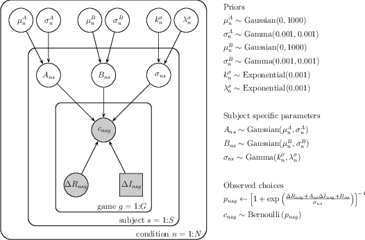
Figure 2 — Graphical depiction of the hierarchical Bayesian model. In this plot, each node corresponds to a variable in the model. Shaded nodes correspond to observed variables (e.g. choices) and unshaded nodes correspond to hidden variables (e.g. information bonus or decision noise). Discrete variables are represented as squares and continuous variables as circles. The group variables, which are illustrated as different “plates,” have different values for different games, g, subjects, s, or conditions, n (defined by the valence, uncertainty and horizon). For each game, the observable data (shaded nodes) consisted of a choice, cnsg, the difference in mean between each option, Δ Rnsg, and the difference in uncertainty between each option, Δ Insg. The model estimates posterior distributions of both the single subject-level parameters: the information bonus, Ans, decision noise, σns, and spatial bias, Bns, and the group-level parameters: µnA, σnA, knσ, λnσ, µnB and σnB.
2.4.2¬Ý¬ÝModel-based analysis
We fit the behavioral data of the first free-choice trial using a logistic model. This model assumes that decisions are made by first computing a noisy value, Qa, for bandit a, and Qb for bandit b, then choosing the option with the highest value. In particular we assume that the value Qa is computed as the weighted sum of four factors: the expected reward from option a, Ra, the uncertainty associated with playing it, Ia, its spatial location (i.e. the bandit on the left vs. the bandit on the right), sa, and a logistic random noise term, n.
In this equation, A denotes bias towards more informative/uncertain options, which for simplicity we call the information bonus, B is the spatial bias, and σd the standard deviation of the decision noise. Ia was chosen such that Ia=+1/2 if option a was the more uncertain option (i.e. the option played once in the forced trials) in the [1 3] condition, Ia=−1/2 if option a was the less uncertain option (the option played three times in the forced trials) in the [1 3] condition, and Ia=0 in the [2 2] condition. sa was set to +1/2 if a was on the left-hand side of the screen and −1/2 if a was on the right.
If we assume that subjects choose the option with highest value and that by convention bandit a is always on the left (for exposition, though not in actuality), then the probability of choosing bandit a is
¬Ý¬Ý
pa¬Ý=¬Ý
1
1+exp(
Œî¬ÝR¬Ý+¬ÝA¬ÝŒî¬ÝI¬Ý+¬ÝB
‚àö
2
σ
)
¬Ý¬Ý¬Ý¬Ý(Eq. 4)
where Δ R = Rb − Ra is the difference between the mean observed outcomes from the forced-choice trials for bandits a and b. Δ I = Ib − Ia is the difference in expected uncertainty from choosing the two options, defined such that Δ I = 0 in the [2 2] equal uncertainty condition, Δ I = +1 in the [1 3] unequal uncertainty condition, when bandit b was more informative than bandit a (i.e. when bandit a had been selected three times and bandit b only once) and Δ I = −1, when bandit a was more uncertain than bandit b. Note that defining Δ I in this way sets A, the information bonus, in units of points.
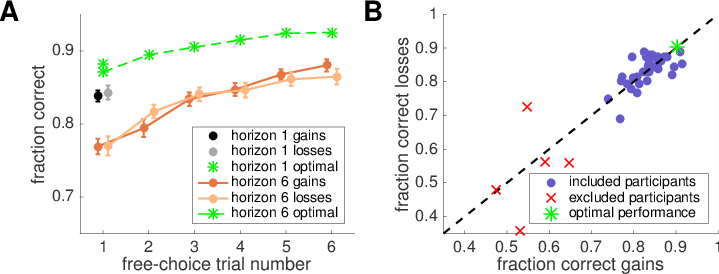
Figure 3 — Performance plots. (A) Learning curves showing the fraction of responses in which subjects (solid lines) and the optimal model (green asterisks) chose the bandit with the greater underlying generative mean, as a function of free-choice trial number. (B) Performance of all 39 subjects in the gains and losses conditions. Five subjects performing at chance in either condition were excluded (red crosses), while the remaining 34 subjects performed equally well in both the gains and losses conditions.
We used a hierarchical Bayesian approach to fit the parameters of the model simultaneously at both the individual and group levels. A graphical depiction of this hierarchical model is shown in Figure 2, using the notation described in Lee and Wagenmakers (2013). At the individual level, we assumed that each subject, s, could have a separate information bonus, Ans, decision noise, σns, and spatial bias, Bns, in each of the eight conditions, n, defined by the valence, uncertainty, and horizon. At the group level, we assumed that these parameters for each subject and condition were sampled from population-level priors. Thus, the information bonus for each condition was sampled from a Gaussian distribution with mean µnA and standard deviation σnA, i.e.
¬Ý
Ans¬Ý‚ຬÝGaussian(¬µnA¬Ý,¬ÝœÉnA)
The decision noise was sampled from a Gamma distribution with shape parameter knσ and length scale λnσ
¬Ý
œÉns¬Ý‚ຬÝGamma(knœÉ,¬ÝŒªnœÉ)
and the spatial bias was sampled from a Gaussian with mean µnB and standard deviation σnB
¬Ý
Bns¬Ý‚ຬÝGaussian(¬µnB¬Ý,¬ÝœÉnB)
The hyperparameters, µnA, σnA, knσ, λnσ, µnB, and σnB are themselves assumed to come from hyperpriors whose parameters are set such that these hyperprior distributions are very broad and have relatively little influence on the final fits. In particular, the means µnA and µnB are assumed to come from zero-mean Gaussian distributions with standard deviation 1000; the standard deviations, σnA and σnB from Gamma distributions with shape parameter 1 and length scale 0.001; the shape and length-scale parameters knσ and λnσ come from Exponential distributions with length scale 0.001.
All parameters (Ans, σns, Bns, µnA, σnA, knσ, λnσ, µnB, and σnB) were fit simultaneously using a Markov Chain Monte Carlo (MCMC) approach to sample from the joint posterior. This was implemented using the JAGS sampler (Plummer, 2003) via the Matjags interface (Steyvers, 2011). In all we ran 4 separate Markov Chains with 500 burn-in steps to generate 1000 samples from each chain with a thin rate of 5. Convergence was assessed through visual inspection (see the Supplementary Material for serial plots of samples).
3¬Ý¬ÝResults
3.1¬Ý¬ÝBasic performance is similar for gains and losses
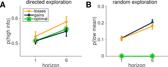
Figure 4 — Model-free measures of directed and random exploration. (A) The fraction of trials in which subjects choose the more uncertain option increases from horizon 1 to horizon 6, indicative of directed exploration. It also increases from gains to losses, but this does not interact with the horizon condition. This is consistent with increased uncertainty seeking in losses, but not a difference in directed exploration between gains and losses. (B) The decision noise (calculated as the fraction of trials in which the low-mean option was chosen) increases from horizon 1 to horizon 6, indicative of random exploration. There is no significant difference in decision noise between gains and losses. Data points are averaged across 34 subjects, with error-bars indicating the standard error of the mean.
We quantified performance as the fraction of times subjects chose the objectively correct option, i.e. the bandit who’s mean was actually highest. As shown in Figure 3A, the group-averaged performance for all subjects (i.e., before eliminating any subjects) was above chance (0.5) in all conditions, with performance improving over the course of horizon 6 games. Subjects were well below optimal performance, but gradually converged toward optimal throughout the course of a horizon 6 game (see the Supplementary Material for an explanation of how we computed optimal behavior).
Out of 39 subjects, the vast majority (34) achieved above chance performance in both valence conditions and performance in one condition was highly correlated with performance in the other (Figure 3B). The five subjects whose performance was at or below chance (as determined by Eq. 2) in one or both conditions were excluded from further analysis.
3.2¬Ý¬ÝDirected and random exploration are equivalent for gains and losses, while uncertainty seeking is increased for losses
To measure the extent of directed exploration, random exploration, and baseline uncertainty seeking we looked at behavior on the first free-choice trial in the Horizon Task in the gains and losses conditions. To give a more complete picture of our data, and to illustrate the robustness of our findings, we performed both a model-free and model-based analysis of the behavior. The model-free analysis is much simpler and is perhaps more intuitive, but comes at the cost of reduced sensitivity and of ignoring variables. The model-based analysis offers more detailed and quantitative insights but at the cost of complexity. Our conclusions are similar for both types of analyses, and some readers may wish to skip the model-based results.
3.3¬Ý¬ÝModel-free analysis
As outlined in the Methods section, we used two model-free metrics to capture directed and random exploration. We computed the fraction of trials in the [1 3] condition in which subjects chose the more uncertain option, p(high info). Because directed exploration involves information seeking, we compared this value across horizons. That is, directed exploration was measured as an increase in p(high info) from horizon 1 to horizon 6, when the information gained from selecting the more uncertain option is useful for future choices. Likewise, because decision noise leads subjects to make “mistakes” we quantified it as the probability of choosing the low mean option in the [2 2] condition, p(low mean). Random exploration was quantified as an increase in p(low mean) from horizon 1 to horizon 6.
A repeated measures ANOVA found a significant increase in p(high info) from horizon 1 to horizon 6 (F(1, 135) = 9.67, p = 0.0039), and from gains to losses (F(1, 135) = 6.00, p = 0.046, one-sided) (Figure 4A). There was no interaction between the valence condition and the horizon condition (F(1, 135) = 0.39, p = 0.54). The increase in p(high info) with horizon is indicative of directed exploration; when subjects are afforded extra trials to explore, they are more likely to choose the more uncertain option in order to gain information about it for future trials. The lack of interaction between valence and horizon indicates that the greater tendency to choose the more uncertain option with losses does not vary across horizons. This horizon-invariant shift towards choosing the uncertain option with losses is consistent with an overall bias toward uncertainty-seeking in the loss domain, but no difference in directed exploration between gains and losses.
For random exploration, a repeated measures ANOVA found a significant increase in p(low mean) from horizon 1 to horizon 6 (F(1, 135) = 56.72, p < 10‚àí8) and no significant difference between gains and losses (F(1, 135) = 1.09, p = 0.30). This increase in decision noise from horizon 1 to horizon 6 is indicative of random exploration as behavioral variability increases when there is opportunity to explore.
3.4¬Ý¬ÝModel-based analysis
To more precisely quantify our findings we used model fitting. We estimated posterior distributions for all parameters in the model for each subject in each condition, using hierarchical Bayesian estimation. For simplicity we focus on the group-level parameters that summarize the group means of the information bonus, µnA, and decision noise, knσ / λnσ. These are shown in Figure 5, with error-bars indicating 95% credible intervals. The spatial bias was near zero across all conditions and is omitted.
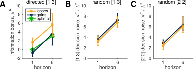
Figure 5 — Model-based measures of directed and random exploration. Parameter fits, averaged across 34 subjects, with error-bars indicating 95% credible intervals across subjects. (A) As with the model-free results, the information bonus is greater in the losses condition than in the gains condition, and greater for horizon 6 than for horizon 1. Decision noise is greater in horizon 6 than in horizon 1 in both uncertainty conditions (B & C), and greater overall in the unequal uncertainty condition (B) than the equal uncertainty condition (C). Decision noise is not significantly different across the gains and losses conditions.
Both the information bonus and the decision noise increased from horizon 1 to horizon 6, in both valence conditions, suggesting that subjects use directed and random exploration for gains and for losses (information bonus and decision noise increased from horizon 1 to horizon 6 in 99.98% and 100% of samples, respectively). Decision noise was not reliably different between gains and losses (greater for losses in 17.8% of samples), and decision noise was greater in the [1 3] unequal uncertainty condition than the [2 2] equal uncertainty condition in 97.4% of samples.
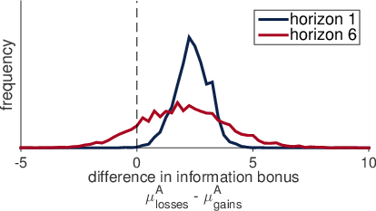
The information bonus was different for gains and losses. In particular there was an overall increase in the bonus in the losses domain (in 98.7% of samples). Thus if we compute the posterior over the difference between the bonus for losses and gains in both horizon conditions (Figure 6) we see approximately the same change between losses and gains in both horizon 1 (losses > gains in 99.8% of samples) and horizon 6 (losses > gains in 88.0% of samples) although the distribution for horizon 6 is broader. The Bayes Factor for our [model versus a model the included an additional information bonus for the losses condition was 0.4997.
There was no interaction between valence and horizon conditions as shown by the fact that the difference in the posteriors for the weight on the more uncertain option in horizon 6 and horizon 1 was identical for both gains and losses (information bonus increased from horizon 1 to horizon 6 in 99.8% of samples from the gains condition, and in 99.6% of samples from the losses condition.).
Figure 6 — Posterior distributions showing the estimated information bonus is greater for losses than for gains. The difference between gains and losses in the posterior distributions of the information bonus shows that the estimated information bonus is greater for losses than for gains. This overall shift in the domain of losses is indicative of uncertainty seeking with losses.
3.5¬Ý¬ÝUncertainty seeking in the losses condition is consistent with Bayesian Shrinkage, not Prospect Theory
The results of both the model-free and model-based analyses revealed an overall bias toward the more uncertain option in the domain of losses. This result is consistent with the classic predictions of Prospect Theory, in which humans seek uncertainty in the domain of losses and avoid uncertainty in the domain of gains. However, our results are also consistent with a Bayesian interpretation that we refer to as the “Bayesian Shrinkage” hypothesis. It should be noted that this Bayesian Shrinkage hypothesis is referring metaphorically to how people do inference, which is distinct from the formal Bayesian statistical analyses presented in this paper (Kruschke 2010; Lee 2011; Lee 2016).
The Bayesian Shrinkage hypothesis assumes that subjects compute the expected value of each option, R, using Bayesian inference with some prior. This prior has the effect of biasing the estimated expected value towards the mean of the prior — it “shrinks” the estimate towards the mean of the prior. Because the effect of the prior is greater on more uncertain options, increased uncertainty seeking in the domain of losses could simply reflect a more optimistic prior, compared to the expectation of the gamble, for losses than for gains.
Intriguingly, despite making similar qualitative predictions about uncertainty seeking with losses, Prospect Theory and Bayesian Shrinkage make different quantitative predictions about the interaction between reward and uncertainty. In the following sections, we describe these predictions in detail and show how our results are consistent with the Bayesian Shrinkage account.
3.6¬Ý¬ÝProspect Theory and Bayesian Shrinkage make different predictions
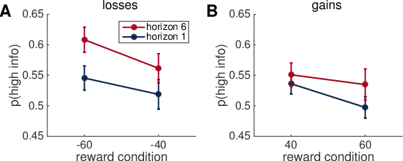
Figure 8 — Model-free analysis of reward magnitude effect is consistent with Bayesian Shrinkage hypothesis. In both horizon conditions, for both losses (A) and gains (B) there is a negative association between mean reward and choice of the more uncertain option, p(high info). Error-bars indicate the standard error of the mean across subjects.
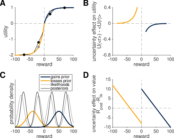
Bayesian Shrinkage explains the change in uncertainty preference between gains and losses by appealing to different prior distributions. If the prior for gains is pessimistic and the prior for losses is optimistic, then these priors cause uncertain options to be undervalued for gains and overvalued for losses (Figure 7C). This in turn leads to uncertainty aversion for gains and uncertainty seeking for losses. The size of the Bayesian Shrinkage effect increases as a function of the difference between the mean of the rewards and the mean of the prior (Figure 7D). This implies a negative relationship between reward and uncertainty seeking for both gains and losses.
Thus, Prospect Theory and Bayesian Shrinkage make opposite predictions about the interaction between uncertainty and reward. Specifically, Prospect Theory predicts an increase in uncertainty seeking with reward, while Bayesian Shrinkage predicts a decrease (Figure 7B, D). These predictions are straightforward to test with our data.
3.7¬Ý¬ÝModel-free and model-based analyses favor Bayesian Shrinkage over Prospect Theory
To distinguish between Prospect Theory and Bayesian Shrinkage in a model-free way, we computed p(high info) separately for high and low reward magnitude trials. To do this we took advantage of the fact that one of the bandits always had a mean of magnitude either 40 or 60 points (see Methods), while the mean of the other bandit was set relative to this. We therefore defined high-magnitude trials as those in which the mean of the main bandit was ±60, and low-magnitude trials as those in which the mean of the main bandit was ±40. The null hypothesis asserts that p(high info) will be independent of the reward level. Prospect Theory asserts that p(high info) will be positively correlated with reward level. Thus, for losses, we expect to see less uncertainty seeking in the –60 than –40 games, while for gains, we expect less uncertainty seeking in +40 than +60 games. The Bayesian Shrinkage hypothesis asserts that p(high info) will be negatively correlated with mean reward, i.e. more uncertainty seeking for –60 than –40 in the losses condition and more uncertainty seeking for +40 than +60 in the gains condition.
We computed p(high info) separately for the eight different magnitude x horizon x valence conditions. The pattern of behavior is consistent with the Bayesian Shrinkage hypothesis with a negative relationship between mean reward and p(high info) (Figure 8A, B). In particular a repeated-measures ANOVA revealed a significant interaction between the gains/losses condition, and the high/low-magnitude condition (F(1, 135) = 10.40, p = 0.0029) in the model-free analysis. There was still a main effect of the valence condition (F(1, 135) = 6.0, p = 0.046, one-sided), and of the horizon condition (F(1, 135) = 9.67, p = 0.0039). There was no main effect of the magnitude condition (F(1, 135) = 0.48, p = 0.49) since it goes in opposite directions for gains and losses. For the losses trials alone, there was a main effect of the low/high-magnitude condition (F(1, 135) = 5.92, p = 0.020), and a trend to this main effect for gains trials alone (F(1, 135) = 3.46, p = 0.072).
For the model-based analysis we added a single factor to our model, an interaction term between uncertainty, Δ I, and mean reward, M. This interaction term allows us to determine whether people are more or less likely to choose the more uncertain option as the mean reward increases and thus distinguish between a Prospect Theory and Bayesian Shrinkage account. More specifically, in this updated model we rewrote the choice probabilities (Eq. 4) as
¬Ý¬Ý
pa¬Ý=¬Ý
1
1+exp(
Œî¬ÝR¬Ý+¬ÝA¬ÝŒî¬ÝI¬Ý+¬ÝŒ≥¬ÝM¬ÝŒî¬ÝI¬Ý+¬ÝB
‚àö
2
σ
)
¬Ý¬Ý¬Ý¬Ý(Eq. 5)
where γ denotes the strength of the interaction term and is predicted to be positive by Prospect Theory and negative by the Bayesian Shrinkage account.
As with the other variables in the model, we assume that γ is sampled from a group-level prior distribution that is potentially different for each subject and each condition. The group-level priors are assumed to be Gaussian with mean µγ and standard deviation σγ. Finally, the hyperparameters, µγ and σγ, are themselves drawn from broad hyperpriors (see Figure S1 for the graphical depiction of this model).
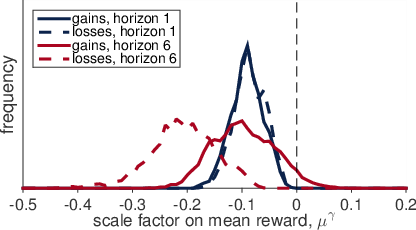
As before, we fit the model using a sampling based approach to compute posterior distributions for all parameters. This clearly shows that the mean of the group-level prior, µγ, is negative in all conditions (Figure 9) with 100% of samples below zero apart from the horizon 6 gains condition where 95.4% of samples are below zero. As discussed above, this negative value is inconsistent with Prospect Theory and provides strong support for the Bayesian Shrinkage hypothesis.
Figure 9 — Distribution of group-level mean of the mean reward scale factor, µγ. In all conditions the µγ is less than zero with high probability, providing strong support for the Bayesian Shrinkage hypothesis.
This model that includes the interaction term was strongly favored over the model without such a term, by 453 points using the deviance information criterion (6,862 for the more sophisticated model versus 7,315 for the more basic model, across 34 subjects). This supports the notion that it is important to account for the interaction between uncertainty and reward.
4¬Ý¬ÝDiscussion
In this study we quantified the effects of reward valence (gains vs. losses) on human explore-exploit decision making. Consistent with our previous work (Wilson et al., 2014), we found evidence that people use two distinct strategies for exploration: directed exploration in which exploration is driven by an increase across horizons in information seeking, and random exploration in which exploration is driven by decision noise that increases with horizon. Moreover, the extent to which subjects used these two strategies was quantitatively comparable in the gains and losses conditions.
In addition we found an overall increase in uncertainty seeking in the domain of losses that initially appeared consistent with the predictions of Prospect Theory (Kahneman et al., 1979; Einhorn et al., 1986; Kahn et al., 1988; Tversky et al., 1992; Di Mauro et al., 1996; Kuhn, 1997; Di Mauro et al., 2002; Ho et al., 2002; Abdellaoui et al., 2005; Du et al., 2005; Baucells et al., 2009; Chakravarty et al., 2009; Davidovichet al., 2009). However, a more detailed, quantitative analysis revealed an interaction between uncertainty and reward magnitude that was inconsistent with Prospect Theory, but that could be explained with the Bayesian Shrinkage hypothesis in which people have a prior that is optimistic for losses and pessimistic for gains.
An obvious question is why do we see this departure from Prospect Theory? One reason may be that, unlike classical tests of Prospect Theory, the uncertainties in our task are not explicitly described but instead must be inferred from experience. A number of authors have found that decisions based on described uncertainties can be quite different from decisions based on uncertainties that are experienced (e.g. Ludvig & Spetch, 2011; Hertwig et al., 2004; Barron & Erev, 2003). However, it is important to note that recent work looking at decisions under ambiguity do not see differences between gains and losses when the decision is made under experience (Dutt et al., 2014; Guney & Newell, 2015). Clearly more work will be required to understand why our experiment gives different results.
One result from the description-experience literature that is inline with our findings is the paper of Teodorescu & Erev (2013) who used an explore-exploit task that combined both gains and losses. In this experiment, the authors found behavior that was consistent with increased uncertainty seeking for losses. However, because losses and gains were always present together — i.e. there were no separate losses-only or gains-only conditions — it was impossible to separate the effects of losses from gains. Our work is also qualitatively consistent with Lejarraga & Hertwig (2016) who found that exploratory behavior in the loss domain was better explained by a simple win-stay/lose-shift heuristic strategy than by loss aversion. While our task, with continuously valued rewards, is not well suited to studying win-stay/lose-shift behavior, it will be important to reconcile these two findings in future work. Finally, our work is consistent with Yechiam, Zahavi & Arditi (2015) who found increased exploration in the domain of losses. Intriguingly, this latter paper also found a hysteresis effect whereby past exposure to losses increased exploration even when the losses where no longer present. Such a long-term effect of past losses may be driven by the “break-even” effect (Thaler & Johnson, 1990) whereby people who have experienced a loss are more likely to choose an uncertain option if it offers the chance to erase the past loss. While our experiment did not offer any possibility of breaking even in the losses condition, future work should examine this idea more closely.
Another task that combines gains and losses in an explore-exploit setting is the Iowa Gambling Task (IGT) (Bechara et al., 1994). In this task, subjects choose between four decks of cards. Each deck contains both winning and losing cards and the relative amount of gains and losses varies between decks such that two decks are winning on average while the other two are losing. In recent years, a number of authors have modeled behavior in this task in detail (e.g. Wetzels et al., 2010; Worth et al., 2013). While the results of these modeling efforts are not directly comparable with our findings here, it would be interesting to include factors for directed exploration and a Bayesian prior in models of the IGT.
At the neural level, a question of particular interest for future work is how these decisions are processed in the brain. Neuroimaging studies have identified areas of the brain involved in value-based decision making (Rangel, Camerer & Montague, 2008; Christopoulos, Tobler, Bossaerts, Dolan & Schultz, 2009; Hare, Camerer & Rangel, 2009; Kahnt, Heinzle, Park & Haynes, 2011), the representation of monetary gains versus losses (Breiter, Aharon, Kahneman, Dale & Shizgal, 2001; Gehring & Willoughby, 2002; De Martino et al., 2006; Yacubian et al., 2006; Seymour et al., 2007; Weller et al., 2007; San Martín et al., 2013), and exploration versus exploitation (Daw et al., 2006; Laureiro-Martínez, Brusoni & Zollo, 2010; Badre, Doll, Long & Frank, 2012). In light of our finding that directed exploration, random exploration, and uncertainty seeking are independent, additive terms in the value computation, neuroimaging could reveal whether these brain regions also function in a summative way under explore-exploit decisions.
Finally, it is important to note that, despite being due to uncertainty seeking rather than exploration, subjects did choose the uncertain, and hence more informative option more in the losses condition of our task. While this did not lead to a significant difference in performance in our experiment (Figure 3), it would be interesting to investigate whether this bias for losses is advantageous in some settings, or whether it is simply a suboptimal bias in human decision making.
References
Abdellaoui, M., Vossmann, F., & Weber, M. (2005). Choice-Based Elicitation and Decomposition of Decision Weights for Gains and Losses Under Uncertainty. Management Science, 51(9), 1384–1399. http://dx.doi.org/10.1287/mnsc.1050.0388.
Aston-Jones, G., & Cohen, J. D. (2005). An integrative theory of locus coeruleus-norepinephrine function: adaptive gain and optimal performance. Annu Rev Neurosci 28, 403.
Badre, D., Doll, B., Long, N., & Frank, M. (2012). Rostrolateral prefrontal cortex and individual differences in uncertainty-driven exploration. Neuron, 73, 595–607. http://dx.doi.org/10.1016/j.neuron.2011.12.025.
Banks, J., Olson, M., & Porter, D. (1997). An experimental analysis of the bandit problem. Economic Theory. 10, 55.
Barron, G., & Erev, I. (2003). Small feedback‐based decisions and their limited correspondence to description‐based decisions. Journal of Behavioral Decision Making, 16(3), 215–233. http://dx.doi.org/ 10.1002/bdm.443.
Baucells, M., & Villasís, A. (2009). Stability of risk preferences and the reflection effect of prospect theory. Theory and Decision, 68(1–2), 193–211. http://dx.doi.org/10.1007/s11238-009-9153-3.
Bechara, A., Damásio, A. R., Damásio, H., Anderson, S. W. (1994). “Insensitivity to future consequences following damage to human prefrontal cortex”. Cognition 50 (1–3): 7–15. http://dx.doi.org/10.1016/0010-0277(94)90018-3.
Bellman, R. (1957). A Markovian decision process (No. P-1066). RAND CORP SANTA MONICA CA.
Breiter, H. C., Aharon, I., Kahneman, D., Dale, A., & Shizgal, P. (2001). Functional imaging of neural responses to expectancy and experience of monetary gains and losses. Neuron, 30, 619–639. http://dx.doi.org/10.1016/S0896-6273(01)00303-8.
Chakravarty, S., & Jaideep, R. (2007). Attitudes towards Risk and Ambiguity across Gains and Losses. In Economic Science Association World Meeting (pp. 1–34). Rome. Retrieved from http://static.luiss.it/esa2007/programme/papers/108.pdf.
Chakravarty, S., & Roy, J. (2009). Recursive expected utility and the separation of attitudes towards risk and ambiguity: an experimental study. Theory and Decision, 66(3), 199–228. http://dx.doi.org/10.1007/s11238-008-9112-4.
Christopoulos, G. I., Tobler, P. N., Bossaerts, P., Dolan, R. J., & Schultz, W. (2009). Neural Correlates of Value, Risk, and Risk Aversion Contributing to Decision Making under Risk. J. Neurosci., 29, 12574–12583. http://dx.doi.org/10.1523/jneurosci.2614-09.2009.
Cohen, J. D., McClure, S. M., & Yu, A. J. (2007). Should I stay or should I go? How the human brain manages the trade-off between exploitation and exploration. Philosophical Transactions of the Royal Society of London. Series B, Biological Sciences, 362(1481), 933–42. http://dx.doi.org/10.1098/rstb.2007.2098.
Davidovich, L., & Yassour, J. (2009). Ambiguity Preference in the Negative Domain. In Conference on Behavioral Economics. Rotterdam.
Daw, N. D., O’Doherty, J. P., Dayan, P., Seymour, B., & Dolan, R. J. (2006). Cortical substrates for exploratory decisions in humans. Nature, 441, 876–879. http://dx.doi.org/10.1038/nature04766.
De Martino, B., Camerer, C. F., & Adolphs, R. (2010). Amygdala damage eliminates monetary loss aversion. Proceedings of the National Academy of Sciences of the United States of America, 107, 3788–3792. http://dx.doi.org/10.1073/pnas.0910230107.
De Martino, B., Kumaran, D., Seymour, B., & Dolan, R. J. (2006). Frames, biases, and rational decision-making in the human brain. Science (New York, N.Y.), 313(5787), 684–7. http://dx.doi.org/10.1126/science.1128356.
Di Mauro, C., & Maffioletti, A. (1996). An Experimental Investigation of the Impact of Ambiguity on the Valuation of Self-Insurance and. Journal of Risk and Uncertainty, 13, 53–71.
Du, N., & Budescu, D. V. (2005). The Effects of Imprecise Probabilities and Outcomes in Evaluating Investment Options. Management Science, 51(12), 1791–1803. http://dx.doi.org/10.1287/mnsc.1050.0428.
Duff, M. O. G. (2002). Optimal Learning: Computational procedures for Bayes-adaptive Markov decision processes (Doctoral dissertation, University of Massachusetts Amherst).
Dutt, V., Arló‐Costa, H., Helzner, J., & Gonzalez, C. (2014). The description–experience gap in risky and ambiguous gambles. Journal of Behavioral Decision Making, 27(4), 316–327. http://dx.doi.org/10.1002/bdm.1808.
Einhorn, H. J., & Hogarth, R. M. (1986). Decision Making Under Ambiguity. The Journal of Business. http://dx.doi.org/10.1086/296364.
Ellsberg, D. (1961). Risk, Ambiguity, and the Savage
Axioms. Quarterly Journal of Economics, 75, 643–669.
Frank, M. J., Doll, B. B., Oas-Terpstra, J., & Moreno, F. (2009). Prefrontal and striatal dopaminergic genes predict individual differences in exploration and exploitation. Nature Neuroscience. 12, 1062.
Gehring, W. J., & Willoughby, A. R. (2002). The medial frontal cortex and the rapid processing of monetary gains and losses. Science (New York, N.Y.), 295, 2279–2282. http://dx.doi.org/10.1126/science.1066893.
Gittins, J. C. (1979). Bandit Processes and Dynamic Allocation Indices. Journal of the Royal Statistical Society, 41(2), 148–177.
Güney, Ş., & Newell, B. R. (2015). Overcoming ambiguity aversion through experience. Journal of Behavioral Decision Making, 28(2), 188–199. http://dx.doi.org/ 10.1002/bdm.1840.
Hare, T. A., Camerer, C. F., & Rangel, A. (2009). Self-control in decision-making involves modulation of the vmPFC valuation system. Science (New York, N.Y.), 324, 646–648. http://dx.doi.org/10.1126/science.1168450.
Hertwig, R., Barron, G., Weber, E. U., & Erev, I. (2004). Decisions from experience and the effect of rare events in risky choice. Psychological science, 15(8), 534–539. http://dx.doi.org/ 10.1111/j.0956-7976.2004.00715.x.
Ho, J. L. Y., Keller, L. R., & Keltyka, P. (2002). Effects of Outcome and Probabilistic Ambiguity on Managerial Choices. Journal of Risk and Uncertainty, 24(1), 47–74.
Kahn, B. E., & Sarin, R. K. (1988). Modeling Ambiguity in Decisions Under Uncertainty. Journal of Consumer Research. http://dx.doi.org/10.1086/209163.
Kahneman, D., & Tversky, A. (1979). Prospect theory: An analysis of decision under risk. Econometrica, 47, 263–292. http://dx.doi.org/10.2307/1914185.
Kahnt, T., Heinzle, J., Park, S. Q., & Haynes, J. D. (2011). Decoding different roles for vmPFC and dlPFC in multi-attribute decision making. NeuroImage, 56, 709–715. http://dx.doi.org/10.1016/j.neuroimage.2010.05.058.
Kass, R. E., & Raftery, A. E. (1995). Bayes Factors. Journal of the American Statistical Association, 90(430), 773–795.
Kruschke, J. K. (2010). What to believe: Bayesian methods for data analysis. Trends in cognitive sciences, 14(7), 293–300.
Kuhn, K. M. (1997). Communicating Uncertainty: Framing Effects on Responses to Vague Probabilities. Organizational Behavior and Human Decision Processes, 71(1), 55–83. http://dx.doi.org/10.1006/obhd.1997.2715.
Laureiro-Martínez, D., Brusoni, S., & Zollo, M. (2010). The neuroscientific foundations of the exploration-exploitation dilemma. Journal of Neuroscience, Psychology, and Economics, 3(2), 95–115. http://dx.doi.org/10.1037/a0018495.
Lee, M.D. (2011). In praise of ecumenical Bayes. Behavioral and Brain Sciences, 34, 206–207.
Lee, M.D. (2016). Bayesian methods in cognitive modeling. To appear in The Stevens’ Handbook of Experimental Psychology and Cognitive Neuroscience, Fourth Edition.
Lee M. D. & Wagenmakers, E. J. (2013). Bayesian Cognitive Modeling: A Practical Course. Cambridge: Cambridge University Press.
Lee, M. D., Zhang, S., Munro, M. N., & Steyvers, M. (2011). Psychological models of human and optimal performance on bandit problems. Cognitive Systems Research, 12, 164–174.
Lejarraga, T., & Hertwig, R. (2016). How the threat of losses makes people explore more than the promise of gains. Psychonomic Bulletin & Review, 1–13.
Lejarraga, T., Hertwig, R., & Gonzalez, C. (2012). How choice ecology influences search in decisions from experience. Cognition, 124(3), 334–342.
Ludvig, E. A., & Spetch, M. L. (2011). Of black swans and tossed coins: is the description-experience gap in risky choice limited to rare events? PloS one, 6(6), e20262. http://dx.doi.org/10.1371/journal.pone.0020262.
Mehlhorn, K., Newell, B. R., Todd, P. M., Lee, M. D., Morgan, K., Braithwaite, V. A., Hausmann, D., Fiedler, K., Gonzalez, C. (2015). Unpacking the exploration-exploitation tradeoff: a synthesis of human and animal literatures. Decision, 2(3), 191–215. http://dx.doi.org/10.1037/dec0000033.
Meyer, R., & Shi, Y. (1995). Choice under ambiguity: Intuitive solutions to the armed-bandit problem. Management Science. 41, 817.
Payzan-LeNestour, E., & Bossaerts, P. (2012). Do not bet on the
unknown versus try to find out more: estimation uncertainty and
“unexpected uncertainty” both modulate exploration. Frontiers in Neuroscience 6, 1
Plummer, M. (2003). JAGS: A program for analysis of Bayesian graphical models using Gibbs sampling. Proceedings of the 3rd International Workshop on Distributed Statistical Computing, F. K. Hornik, ed. (Technische Universität Wien, Vienna, Austria, 2003).
Rangel, A., Camerer, C., & Montague, P. R. (2008). A framework for studying the neurobiology of value-based decision making. Nature Reviews Neuroscience, 9(7), 545–56. http://dx.doi.org/10.1038/nrn2357.
San Martín, R., Appelbaum, L. G., Pearson, J. M., Huettel, S. a, &
Woldorff, M. G. (2013). Rapid brain responses independently predict
gain maximization and loss minimization during economic decision
making. Journal of Neuroscience, 33,
7011–9. http://dx.doi.org/10.1523/JNEUROSCI.4242-12.2013.
Seymour, B., Daw, N., Dayan, P., Singer, T., & Dolan, R. (2007). Differential encoding of losses and gains in the human striatum. The Journal of Neuroscience, 27, 4826–4831. http://dx.doi.org/10.1523/JNEUROSCI.0400-07.2007.
Steyvers, M., Lee, M., & Wagenmakers, E. (2009). A Bayesian analysis of human decision-making on bandit problems. Journal of Mathematical Psychology 53, 168.
Teodorescu, K., & Erev, I. (2013). On the Decision to Explore New Alternatives: The Coexistence of Under- and Over-exploration. J. Behav. Dec. Makinghttp://dx.doi.org/ 10.1002/bdm.1785..
Thaler, R. H., & Johnson, E. J. (1990). Gambling with the house money and trying to break even: The effects of prior outcomes on risky choice. Management science, 36(6), 643–660.
Tversky, A., & Kahneman, D. (1992). Advances in prospect theory: Cumulative representation of uncertainty. Journal of Risk and Uncertainty, 5, 297–323. http://dx.doi.org/10.1007/BF00122574.
Weller, J. a, Levin, I. P., Shiv, B., & Bechara, A. (2007). Neural correlates of adaptive decision making for risky gains and losses. Psychological Science, 18(11), 958–64. http://dx.doi.org/10.1111/j.1467-9280.2007.02009.x.
Wetzels, R., Vandekerckhove, J., Tuerlinckx, F., & Wagenmakers, E. J. (2010). Bayesian parameter estimation in the Expectancy Valence model of the Iowa gambling task. Journal of Mathematical Psychology, 54(1), 14–27.
Wilson, R. C., Geana, A., White, J. M., Ludvig, E. A., & Cohen, J. D. (2014). Humans use directed and random exploration to solve the explore- exploit dilemma. Journal of Experimental Psychology: General. Advance online publication. http://dx.doi.org/10.1037/a0038199.
Worthy, D. A., Hawthorne, M. J., & Otto, A. R. (2013). Heterogeneity of strategy use in the Iowa gambling task: a comparison of win-stay/lose-shift and reinforcement learning models. Psychonomic bulletin & review, 20(2), 364–371.
Yacubian, J., Gläscher, J., Schroeder, K., Sommer, T., Braus, D. F., & Büchel, C. (2006). Dissociable systems for gain- and loss-related value predictions and errors of prediction in the human brain. The Journal of Neuroscience, 26, 9530–9537. http://dx.doi.org/10.1523/JNEUROSCI.2915-06.2006.
Yechiam, E., Zahavi, G., & Arditi, E. (2015). Loss restlessness and gain calmness: durable effects of losses and gains on choice switching. Psychonomic bulletin & review, 22(4), 1096–1103.
Zhang, S., & Yu, A.J. (2013). Forgetful Bayes and myopic planning: Human learning and decision making in a bandit setting. Advances in Neural Information Processing Systems 26, 2607–2615.
Department of Psychology, Princeton University 08544.
This research was made possible through the support of a grant from the John Templeton Foundation. The opinions expressed in this publication are those of the authors and do not necessarily reflect the views of the John Templeton Foundation. The authors would like to thank the reviewers and the editor for their feedback, which substantially improved this paper.
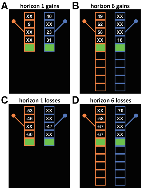 Figure 1 — Task design. Screenshots of four different games showing the gains condition (A & B) and losses condition (C & D), and the horizon 1 condition (A & C) and horizon 6 condition (C & D). In the gains condition, points are added to subjects’ scores, and in the losses condition, points are subtracted. The height of the bandits represents the game length, either 5 or 10 trials. The first four trials of every game are forced, wherein subjects are instructed which bandit to select. In the [1 3] unequal uncertainty condition illustrated here, subjects are instructed to choose one option once and the other three times. In the [2 2] equal uncertainty condition, not shown, subjects play both options twice. Free-choice trials are cued by a pair of green squares located inside the box of each bandit. Once a subject presses a button to choose a bandit, the lever of that bandit flips down and the number of points for that bandit is displayed, followed by the onset of any remaining free-choice trials.