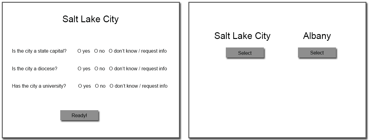
| Figure 1: Learning task (left) and decision task (right). |
Judgment and Decision Making, Vol. 9, No. 1, January 2014, pp. 35-50
Cognitive integration of recognition information and additional cues in memory-based decisionsAndreas Glöckner* Arndt Bröder# |
Glöckner and Bröder (2011) have shown that for 77.5% of their participants’ decision making behavior in decisions involving recognition information and explicitly provided additional cues could be better described by weighted-compensatory Parallel Constraint Satisfaction (PCS) Models than by non-compensatory strategies such as recognition heuristic (RH) or Take the Best (TTB). We investigate whether this predominance of PCS models also holds in memory-based decisions in which information retrieval is effortful and cognitively demanding. Decision strategies were analyzed using a maximum-likelihood strategy classification method, taking into account choices, response times and confidence ratings simultaneously. In contrast to the memory-based-RH hypothesis, results show that also in memory-based decisions for 62% of the participants behavior is best explained by a compensatory PCS model. There is, however, a slight increase in participants classified as users of the non-compensatory strategies RH and TTB (32%) compared to the previous study, mirroring other studies suggesting effects of costly retrieval.
Keywords: parallel constraint satisfaction, probabilistic inferences,
recognition, strategy classification, decision time, confidence.
How do people integrate different pieces of information to draw inferences about unknown criterion variables? For example, how do they infer which of two cities has the higher population? How do they infer which of two exotic bugs is more poisonous? Or how do they decide which of two desserts has more calories? In judgment and decision research, there is wide agreement that summary evaluations or inferences are arrived at by considering pieces of evidence (cues) or attributes of the decision objects (e.g., Brunswik, 1955; Doherty & Kurz, 1996; Karelaia & Hogarth, 2008). For example, individuals will monitor the size as well as the cream and sugar content of a dessert to assess its calories. However, there is less agreement on how this cue information is processed. Whereas traditional approaches assumed a full compensatory integration of available information (e.g., Brehmer, 1994), the simple heuristics framework put forward by Gigerenzer, Todd, and the ABC Research Group (1999) challenged this view and pointed to various simple heuristics that operate only on subsets of available information. Despite their ignoring of information, these heuristics have been shown to be surprisingly accurate and robust in a variety of environments (e.g., Czerlinski, Gigerenzer, & Goldstein, 1999; Davis-Stober, Dana, & Budescu, 2010; Hogarth & Karelaia, 2007; Todd & Gigerenzer, 2012). One particularly frugal strategy is the Recognition Heuristic (RH) promoted by Goldstein and Gigerenzer (2002). If you encounter two objects and recognize only one of them, then infer that the recognized object scores higher on the to-be-judged criterion. This simple strategy works well in domains where recognition is correlated with the criterion (e.g., city sizes, mountain heights, turnover rates of companies), and it has been proposed as a psychological model for these situations. However, the non-compensatory nature of RH (people rely exclusively on recognition) has been debated extensively (e.g., Bröder & Eichler, 2006; Hilbig, Erdfelder, & Pohl, 2010; Marewski, Pohl, & Vitouch, 2010, 2011a, 2011b; Newell, 2011; Newell & Fernandez, 2006; Pachur & Hertwig, 2006; Pachur, Todd, Gigerenzer, Schooler, & Goldstein, 2011, 2012; Pohl, 2011), and studies demonstrating the compensatory use of additional cue knowledge have helped to delineate the conditions under which RH might be used (see Goldstein & Gigerenzer, 2011; Gigerenzer, Hertwig & Pachur, 2011).
The experiment reported in this article pits the recognition heuristic and a sophisticated Take-The-Best (TTB) heuristic in a city size task against the parallel constraint satisfaction model (PCS; Glöckner & Betsch, 2008a) which assumes a compensatory automatic integration of all available cue information. It is an improved follow-up experiment to that of Glöckner and Bröder (2011), which had been criticized by Goldstein and Gigerenzer (2011) for using an inferences from givens paradigm for which RH had not be formulated in the first place. Hence, the current experiment is important in extending the model comparison to memory-based inferences, thus fulfilling one major methodological desideratum for testing the RH against other models.
The current article is organized as follows: First, we will briefly summarize the debate on the alleged noncompensatory use of recognition information, including increasingly sophisticated methodological requirements. Second, we will introduce PCS and summarize the results from Glöckner and Bröder (2011) as well as the criticism by Goldstein and Gigerenzer (2011). Finally, we will present the results of the new study and discuss how this further delineates RH’s range of applicability as a psychological model.
RH’s appeal as a cognitive model of inferences under partial ignorance stems from convincing demonstrations that it can be quite accurate in situations where the validity of the recognition cue is high (e.g., Goldstein & Gigerenzer, 2002). Further, all studies up to now examining the use of recognition information in situations with high recognition validity demonstrated that this meta-cognitive cue is indeed relied upon heavily in probabilistic inferences. The importance of this novel discovery notwithstanding, some stronger claims proposed by Goldstein and Gigerenzer (2002) have been apprehended with more skepticism.
One example is the prediction concerning objects that “may be recognized for having a small criterion value. Yet even in such cases the recognition heuristic still predicts that a recognized object will be chosen over an unrecognized object.” (Goldstein & Gigerenzer, 2002, p. 76). Oppenheimer (2003) took the challenge to test this claim by having people decide between unknown (fictitious) cities with Chinese-sounding names and well-known small cities, and he found that people did not follow the RH in these cases, thus falsifying this specific prediction which is therefore not seen as an essential feature of RH anymore (Gigerenzer, Hertwig, & Pachur, 2011, p. 59). Pachur and Hertwig (2006) termed these situations in which RH use is not expected as those involving “conclusive criterion knowledge” (see also Pachur, Bröder, & Marewski, 2008; Hilbig, Pohl, & Bröder, 2009).
A more prominent controversial prediction is the noncompensatory use of the RH, described by Goldstein and Gigerenzer (2002, p. 82) as follows: “The recognition heuristic is a noncompensatory strategy: If one object is recognized and the other is not, then the inference is determined; no other information about the recognized object is searched for and, therefore, no other information can reverse the choice determined by recognition.” Numerous experiments have tested this claim and found counterevidence (Bröder & Eichler, 2006; Hilbig & Pohl, 2009; Newell & Fernandez, 2006; Newell & Shanks, 2004; Pohl, 2006).1 These studies all suggested that some further available cue information is integrated into the judgments in addition to or instead of mere recognition (although alternatives to RH are not directly tested). However, after the fact, most of these studies were criticized as violating one or more alleged preconditions of RH. For example, some studies used a paradigm in which cue information was available on the computer screen during decision making (e.g., Newell & Shanks, 2004), whereas the RH is formulated for memory-based decisions. Other studies induced recognition by repeated confrontation with stimuli that had been unrecognized before (e.g., Bröder & Eichler, 2006; Newell & Shanks, 2004) rather than relying on “naturally” recognized objects. Or, the RH was tested in environments with demonstrably low recognition validity (Richter & Späth, 2006). Pachur et al. (2008) summarize and discuss several of these methodological caveats (see their Table 1). Their own Experiment 3 tried to come close to the ideal of a fair test of the RH by (a) avoiding induced object and cue knowledge, by (b) relying on memory-based decisions, (c) using the city size task with recognition validity known to be high, (d) controlling for the nature of additional cue knowledge, and (e) by not providing cue information for unrecognized objects. As a dependent variable, Pachur et al. (2008) assessed the proportion of trials in which an individual made choices compatible with RH’s prediction (see Hilbig, 2010; Hilbig et al., 2010, for critiques). At the group level, Pachur et al. could show a significant influence of the nature and amount of cue knowledge participants had about the recognized cities, thus clearly ruling out that all participants used recognition information in a noncompensatory fashion. However, at the level of individual participants, 50% of them never departed from RH’s prediction and always chose the recognized over the unrecognized object. Hence, at least 50% of Pachur et al.’s participants may have used the RH consistently.
However, the merely outcome-based adherence rate does not allow for strict conclusions about the cognitive processes involved: A perfect adherence to RH may occur even when a person considers all available cue information, but the available “conflicting” cues never suffice to overrule the weight of the recognition cue. Hence, the adherence rate at the individual level cannot tell us whether someone used the RH even if it perfectly conforms to RH. On the other hand, even if adherence is not perfect, this could also be explained by unsystematic lapses if someone consistently uses RH!2 Hence, adherence rates are only ambiguous evidence for or against RH use (Hilbig, 2010).
The ambiguity of mere choice outcome data in assessing decision strategies led Glöckner and Bröder (2011) to include reaction times and confidence ratings as further dependent variables in their experiment. Although different heuristics and strategies will often predict identical choices (depending on the subjective weighting of cues), the different cognitive mechanisms can be differentiated by varying predictions for response times and confidence judgments across different item types. These dependent variables can be analyzed simultaneously in the Multiple-Measure Maximum Likelihood (MM-ML) approach (Glöckner, 2009, 2010; Jekel, Nicklisch, & Glöckner, 2010) by determining the joint likelihood of choices, response times, and confidence judgments under each competing model. The MM-ML approach is described in detail in Appendix B. Participants are classified as users of the strategy which produces the highest joint likelihood of the data. However, to derive model predictions, it is necessary to have experimental control over the cues participants might possibly include in their judgments.
In their study, Glöckner and Bröder (2011) had German participants compare the population sizes for 16 medium-sized American cities in a full paired comparison (120 trials). Eight of these cities were mostly recognized, the other eight cities were mostly unrecognized according to a pilot study.3 Both sets of cities comprised all possible patterns of 3 binary cues (state capital, diocese, major university). Note that the cue values were veridical, so no invalid information was ever presented to the participants. During the decision phase, participants were provided with the city names along with the cue patterns (in a matrix format containing “+” and “-” for positive and negative cue values, respectively). They chose one of the cities as the more populous, and response times were recorded. Each trial was followed by a confidence assessment.
The goal of the study by Glöckner and Bröder (2011) was to assess the strategies participants would use in such a task, pitting RH, TTB and two variants of the PCS model against each other. For RH it was assumed that, in cases where one object is recognized and the other is not, people would rely exclusively on the recognition cue without considering further information. In case of a non-discriminating recognition cue, we expected that participants commence in a TTB-like manner (that is, going through the attributes in a fixed order of decreasing validity until one of them discriminates the two options; see Gigerenzer & Goldstein, 1996). TTB in our version did not necessarily consult the recognition cue first, but it searched recognition and the other cues in order of decreasing subjectively estimated validity until one discriminating cue was found on which the decision could be based. Hence, TTB and RH could both be applied to any comparison between cities, including decisions between cities that were both known or unknown and strategy predictions could still differ. The PCS model by Glöckner and Betsch (2008a) is a network model in which activation spreads through the network until a stable and consistent representation is found (e.g., Holyoak & Simon, 1999; McClelland & Rumelhart, 1981; Read, Vanman, & Miller, 1997; Simon, Snow, & Read, 2004; Thagard & Millgram, 1995). All cues are processed in parallel, and reaction time predictions can be derived from the number of cycles the network needs to settle in the stable state. In contrast to RH and TTB, PCS is a fully compensatory model which includes all available cue information. Confidence judgments are predicted by comparing the final activation of both option nodes.
Details about the network specifics are provided in Appendix A, and recent developments can be found in several current publications (e.g., Betsch & Glöckner, 2010; Glöckner & Betsch, 2012; Glöckner & Bröder, 2011). Although the PCS model is an overarching single-strategy model, it allows for taking into account individual differences in sensitivity to cue validities. This difference can potentially be captured by a continuous parameter, but Glöckner and Bröder (2011) used the strategy in a low (i.e., PCS1) and a high (i.e., PCS2) cue-sensitivity implementation only.4
According to the MM-ML classification taking into account the full set of 120 tasks (including comparisons between two recognized or two unrecognized cities), 77.5% of the participants appeared to follow a PCS model (either PCS1 or PCS2), whereas the remaining 22.5% of participants were classified as using one of the two noncompensatory strategies RH or TTB. These results suggested that the noncompensatory strategies played only a minor role in this paradigm. Note, however, that the result does not imply that people did not rely on the recognition cue, but they did obviously not rely on it exclusively. The pattern of response times and confidence judgments across items favored the interpretation that the other cues were used as well. The results furthermore showed that it is useful to take individual differences in cue-sensitivity in PCS into account, given that participants were classified in both categories (i.e., PCS1: 47.5% and PCS2: 30%).
In using natural recognition, stimuli without conclusive criterion knowledge, a domain with high recognition validity, control of additional cue knowledge, and real (rather than artificial) stimuli, Glöckner’s and Bröder’s (2011) experiment fulfilled five of the eight ideal preconditions formulated by Pachur et al. (2008) that may foster the use of RH. In addition, the study aimed at model comparisons rather than just refuting claims of the RH. This was also a desideratum formulated by researchers favoring the fast and frugal heuristics approach (Marewski, Gaissmaier, et al., 2010; Marewski, Schooler, & Gigerenzer, 2010).
In order to derive precise model predictions, people were provided with cue values of the decision objects in the lab, also for the unrecognized cities. Furthermore, decisions were screen-based (i.e., cue information was presented on screen) rather than memory-based. In the current study we again provide cue values for unrecognized objects and we will come back to this potential issue of debate in the discussion. The second point concerning screen-based decisions was criticized by Goldstein and Gigerenzer (2011) as the main weakness of the study, neglecting a major boundary condition of RH use. Therefore, the current study addresses this major shortcoming and investigated inference decisions from memory rather than from givens. This is also important because evidence reported by Glöckner and Hodges (2011) indicates that the prevalence of PCS seems to be reduced in memory-based decisions. In a similar vein, results from Söllner, Bröder, and Hilbig (2013) suggest that usually high prevalence rates for PCS in decisions from screen are reduced if the presentation formats differs from the matrix-like presentation format used by Glöckner and Bröder (2011). Therefore, the current experiment is another important step in delineating the conditions of RH use. Using the common paradigm introduced by Bröder and Schiffer (2003b) to investigate memory-based decisions, we had participants learn cue values of different natural objects (American cities) by heart before the decision phase. Hence, participants might later retrieve this information from memory to reach their decisions, or they might rely solely on the recognition cue.
We investigated the use of recognition information in inferences from memory. Thereby, the paradigm used in Glöckner and Bröder (2011) was extended by adding a learning phase in which participants acquired cue information. In the learning phase, participants were presented with three pieces of information about each of 16 American cities, approximately half of them being known and half of them being unknown. The same stimuli as in Glöckner and Bröder (2011) were used. Afterwards participants decided in an incentivized task repeatedly which of two of these American cities has more inhabitants. For this decision they were not provided with any information but they could potentially retrieve information from memory. However, they could also rely on recognition exclusively or search cues sequentially in accordance with TTB, ignoring some of the information (Bröder & Gaissmaier, 2007; but see also Bröder & Schiffer, 2003b; Bröder & Schiffer, 2006).
Figure 1: Learning task (left) and decision task (right).
Sixty-one students of different subjects took part in the experiment (37 female, mean age 23.8 years). The experiment lasted about 50 minutes. Participants received performance-contingent payment between 4.53 Euros and 11.83 Euros for the study. No between-subjects manipulation was used but the structure of the decision task was manipulated within subjects (see below).
We used the materials from Glöckner and Bröder (2011), which consisted of 2 sets of 8 mid-size US-American cities between 50.000 and 300.000 inhabitants which were mainly known or mainly unknown, respectively.5 The cities were selected so that they had specific properties concerning the cues used in this study which were: a) is the city a state capital or not? b) is the city a diocese / does it have a bishop or not? c) does the city have a major university (with more than 4000 students) or not? Cities were selected so that they represented all eight possible (i.e., 23) cue combinations for known cities as well as for unknown cities. The 16 times 3 (= 48) pieces of information for the cities were learned in the learning phase. All 16 cities were compared to each other in the main experiment resulting in 120 decision tasks.
The learning phase and the decision phase were presented to the participants as two separate experiments. Participants were first informed only about an incentivized task to learn information about American cities. They were informed about the decision tasks only after they had successfully completed this learning phase. Participants were informed that it would take several learning trials to reach the threshold of 90% correct knowledge. Each trial consisted of a learning part and a test part. In the learning part the 16 cities were presented in random order and the participants could ask for information about each cue value or directly indicate the cue values. Only after all three pieces of information for one city were indicated correctly was the next city shown. In the test phase all cities were presented in random order, the participants indicated each cue value and received feedback whether the values were correct. At the end of the test phase participants received feedback about their learning performance. If the performance was above 90% correct they continued with the test phase. The learning phase was aborted after 30 min. Specifically, participants entered the decision phase after finishing the respective learning trial in which they crossed the time-deadline. The learning phase was incentivized in that participants could receive up to 5 Euros for reaching this threshold quickly and with as few errors as possible.6
In the decision phase, participants were informed that they should make decisions concerning which of two US-American cities has more inhabitants and that they would receive 10 Cent for each correct answer and lose 1 Cent for each wrong answer. The city names were presented on the screen without any further information and choices were indicated by mouse-click. Participants received feedback concerning the correctness of their choices only at the end of the experiment. They were informed that in case there are different US-cities with the same name, the larger one is referred to. Finally, they were introduced to the confidence measure which was presented after the decision and they were instructed to make good decision and to proceed as fast as possible. Participants solved a warm-up trial. If there were no more questions, participants started working on the 120 decisions, which were presented in individually randomized orders. The presentation order of the two cities on each screen (i.e., left / right) was also randomized. Confidence was measured on a scale from very uncertain (-100) to very certain (100) using a horizontal scroll-bar. Decision trials were separated by blank screen with a continue button. A pause screen announcing a voluntary 1-minute-break was presented after half of the tasks to reduce effects of decreasing attention.
After the choices were completed we measured participants’ cue-usage, cue order, and perceived cue-validity. First, participants indicated how much they relied on each of the three cues when making their decision and how much they relied on whether they knew the city before on a scale from not used (0) to very much used (100). Participants indicated which of the four pieces of information (3 cues plus recognition of the city) predicts the size of US-cities best by ranking the four pices (i.e., assigning numbers between 1 and 4). Participants were asked about their prior knowledge about the cities on a three point scale (1-unknown, 2-I knew the name, 3-I knew more than the name). Finally we measured subjective estimations of cue-validities directly by asking participants to indicate how many of 100 US-cities with the respective property are larger than cities without it for the three cues and recognition using a horizontal scroll-bar (scale: 50-100).
Participants were successful in acquiring cue information. The average rate of correctly reproduced cue information in the last test phase was 90%. Most participants (61%) reached the criterion of 90% correct answers, the others came close to it. Also our manipulation of recognition was efficient. For the eight “unknown cities” across participants we found that 76% of them were indeed unknown. For the “known cities” we found that 87% were known. Each “unknown city” was unknown to the majority of the participants and the reverse was true for the “known cities”. Individuals’ explicated cue-hierarchies (according to the ordering of the predictive power of the information) were very heterogeneous. Most participants said that state capital (43%) or recognition (43%) is the best predictor whereas much less indicated diocese (2%) or university (13%). A similar order was found in the subjective numerical cue-validity ratings (in the same order with SE in parentheses): 80 (1.8), 76 (2.0), 57 (1.1), and 75 (1.6); and in the subjective cue-usage rating: 71 (3.8), 70 (3.7), 23 (2.7), and 60 (4.3). Participants were rather consistent in their answers to all three measures. Order of cues correlated highly negative with cue usage (Md(ρ ) = −.80) and cue validity (Md(ρ ) = −.80); and the latter also correlated highly with each other (Md(ρ ) = .80).
Figure 2: Mean proportion of correct choice predictions for each of the 120 decision tasks (dots) plotted against each other for the considered strategies. 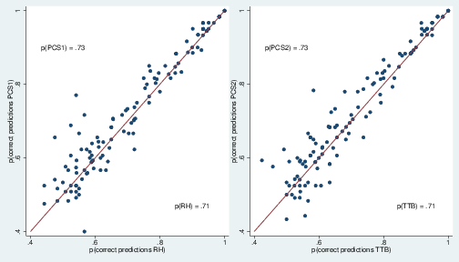
We calculated strategy predictions for RH, TTB, and the two versions of PCS (i.e., PCS1: low sensitivity to differences in cue validities = cue usage transformation linear; PCS2: high sensitivity = cue usage transformation quadratic) for the 120 decision tasks concerning choices, decision time and confidence in the same manner and with the same parameters as in Glöckner and Bröder (2011). PCS with two sets of parameters was used to take into account individual differences in sensitivity to cue validities and to put PCS and the heuristic toolbox on equal footing concerning flexibility. Details concerning PCS and the other strategies are described in Appendix A. We again took into account individuals’ cue hierarchies (based on ratings of subjective cue usage) and individuals’ true recognition of cities. The only difference was that we also took into account the acquired cue knowledge instead of the true cue values, in that we set all cue values that individuals were not able to correctly report in the last learning test to 0 (i.e., no cue information). This individualization of choices occasionally led to inconclusive comparisons (no strategy predictions possible in 3.5% of the cases), which were excluded from the analysis.
The two versions of PCS predicted on average 73% of the choices correctly, whereas RH and TTB predicted 71% correctly. Figure 2 plots proportion of correct predictions for the 120 decision tasks comparing PCS1 against RH (left) and PCS2 against TTB (right). Each dot indicates one comparison of two cities and the axis provide the proportion of participants that chose in line with the prediction of the strategy for this task. Dots above the 45 degree line indicate that for the respective decision task the PCS models prediction was correct for more participants than the RH/TTB prediction (and vice versa for dots below the line). Note that the specific selection of the strategy pairings is arbitrary and does not follow a special logic except that PCS strategies should be paired with heuristics.
Figure 3: Mean observed decision times (y-axis) for each of the 120 decision tasks (dots) plotted against the interval scaled predictions (x-axis) of each strategy (different plots). Note. Predictions of RH and TTB for each choice are derived from the number of cues needed to differentiate between options (range 1 to 4). The predictions of PCS are derived from the number of activation updating cycles that network needs to settle in a coherent state (typical range 80 to 180 cycles).
Participants followed the instruction and made rather quick decisions (M = 3316 ms, sd = 2973 ms, Md = 2287 ms, Skew = 4.4, Kurt = 43.4). To reduce skewness and the influence of outliers, decision times were log-transformed, and, to correct for learning order effects, the trial number was partialled out for further analyses (see Glöckner, 2009, p. 197). To investigate at an aggregated level whether the time predictions of the different strategies fit with observed decision times, we compare predicted time and observed time scores (i.e., time-residual after log-transformation and partialling out order effects) of all 120 decision tasks, averaged across participants. Figure 3 shows that the two version of PCS1 were much better able to predict average decision time observed in the 120 tasks than RH and TTB.
Figure 4: Mean observed confidence ratings (y-axis) for each of the 120 decision tasks (dots) plotted against the interval scaled predictions (x-axis) of each strategy (different plots). Note. Predictions of RH and TTB for each choice are derived from the validity of the discriminating cue in percent and can range from 50 to 100. The predictions of PCS are derived from difference in activation between option nodes in the network and can range from −2 to 2.
As in Glöckner and Bröder (2011), participants indicated that they were not very confident in their decisions and showed high variance, M = 14.7, sd = 47.9 (scale: −100 to 100). To analyze whether confidence predictions of the different strategies fitted to the observed confidence measures we again compared predictions and data after averaging for each of the 120 decision tasks across participants. Again, the two versions of PCS predicted the pattern of confidence better than RH and TTB (Figure 4).
Figure 5: Strategy use based on multiple measure maximum likelihood strategy classification. Note. Bars with labels containing multiple-strategy (e.g., “TTB/RH”) indicate that behavioral data were equally likely for both strategies.
As in Glöckner and Bröder (2011), to investigate strategies at an individual level, we analyzed the overall behavioral data simultaneously (i.e., choices, confidence, and response time) using a Multiple-Measure Maximum Likelihood (MM-ML) strategy classification method (Glöckner, 2009, 2010; Jekel et al., 2010), which is described in more detail in Appendix B. We again take into account the full vector of behavioral observations from all choice tasks (i.e., 120 choices, 120 response times, 120 confidence ratings per participant) and compare them against the predictions of each strategy. As can be seen in Appendix B, the (maximum) likelihood for the total data vector is calculated as product of three components. The first component is the likelihood for observing the pattern of choices assuming a constant application error according to a binomial distribution as suggested by Bröder and Schiffer (2003a). The second and third component are likelihoods that follow from regressing observed decision time and confidence on the respective strategy predictions according to standard maximum-likelihood regressions assuming normally distributed residuals. Hence, conceptually MM-ML integrated two correlations for response time and confidence and a fit index for choices into one overall measure weighting all of them equally. Doing so by simultaneously considering choices, decision times and confidence in MM-ML leads descriptively to a majority of classification of PCS users (62%) and fewer users of noncompensatory strategies (32%) (Figure 5). Note that equal fits of RH and TTB were classified as RH/TTB meaning that either model could fit the data equally well. There were four persons classified as random choosers and one person could not be classified (not reported in Figure 5).
The reliability of MM-ML strategy classification can be evaluated by inspecting error rates and the Bayes factor. We found that average estimated error rates for strategy application of the strategies were between 21 and 26%. Error rates were on average higher than in decisions from givens (Glöckner & Bröder, 2011: 14 to 28%), which might be explained by memory errors and has been observed in memory-based experiments before (Bröder & Schiffer, 2003b). The Bayes-factors (comparing the likelihood of the best and the second best strategy) were a bit lower than in previous research (Md(BF) = 6.6) indicating a moderate reliability of strategy classification. Adding a global misfit-test (Moshagen & Hilbig, 2011) did not influence the results in that the distribution of strategies remained the same and no previous user of a systematic strategy had to be excluded.
For robustness checks we also analyzed results using cue-validities instead of cue-usage as cue weights in PCS1 and PCS2 (w = ((v−50)/100)1; w= ((v−50)/100)2) as done in some other work (Glöckner & Betsch, 2012). Results concerning strategies remained qualitatively the same (56% PCS1 & 2; 37% TTB & RH) although there were some shifts within each category. Interestingly, strategy classification was more reliable in this specification as indicated by a higher median BF = 26.3.
In a second step, we analyzed whether results change if we do not replace wrongly remembered cue values by 0 in generation of model predictions but use the cue values that people reported in the memory test. This did not change the qualitative pattern of results for strategy classification (54% PCS1 & 2; 37% TTB & RH) but tended to reduce strategies ability to predict decision time, confidence as well as choices. Hence, based on these findings, it seems more appropriate to represent unavailable cue information as missing values.
Third, we tested whether strategy classification depended on individuals’ learning rate in the learning phase. The results were again robust in that the relative distribution of strategies remained the same (i.e., more than 60% PCS users) when excluding participants with learning rates below 70%, 80% or 90%.
Furthermore, for the conclusions to be valid it has to be assured that none of the strategies is put at a systematic disadvantage in the analysis. One potential issue concerns decision time predictions. Decision time will clearly be influenced not only by the time necessary to integrate the information. It will also depend on the time required for retrieving cue information. That is, for the recognition cue, it will be important how long it takes to recognize that a city is known or not. For the other cues, decision time will be influenced by the time it takes to activate or retrieve them from memory (if they are used). Both factors are not taken into account in the implementation of the strategies considered here. Hence, correlations between model predictions and observed decision time underestimate the true relation. Given that the variance for recognition and cue activation can be assumed to be additive, strategies that take into account more information will be affected more strongly by the problem than strategies that consider less information. For the RH, for example, recognition information has to be retrieved only but for the PCS strategies recognition information and all other cues have to be retrieved. PCS strategies are therefore put at a disadvantage. Given that PCS still clearly accounted better for decision times this influence seems to be not crucially important. To check the robustness of our findings, we still reran the MM-ML analysis without decision time, including choices and confidence only. The results remained the same (60% PCS1 & PCS2, 33% RH & TTB).
Finally, we investigated the effect of dropping confidence and decision time data and analyzing choices only. We found that the majority of persons was not uniquely classifiable to one strategy or they were classified as user of a random strategy (52%). From the remaining participants there were 19 persons classified as RH or TTB and 10 classified as PCS.
The study reported here rectified what has been criticized as the major shortcoming of the study by Glöckner and Bröder (2011) comparing the ability of RH, TTB, and PCS to explain probabilistic inference decisions. Instead of using a screen-based design and providing cue information during the decision process, all judgments investigated in the current study were memory-based. Nevertheless, the results were quite similar to the former study: The majority of participants was best described by a compensatory PCS model, whereas a minority could be classified as using RH or TTB. Still, when comparing across studies, the prevalence of users of non-compensatory strategies was somewhat increased (but see below) when using memory-based decision as compared to the screen-based decisions (see Glöckner & Bröder, 2011). Both findings resonate with results from Glöckner and Hodges (2011) who focused on the comparison of TTB and PCS, however. Interestingly, even the distribution of participants over the two versions of PCS could be replicated. As in Glöckner and Bröder (2011), although there were considerable individual differences, more participants were classified as users of PCS strategy with lower (i.e., PCS1) as compared to higher (i.e., PCS2) sensitivity to differences in cue validities. Note, that this is the case although PCS2 has been shown to more closely approximated the naïve Bayes solution (Jekel, Glöckner, Fiedler, & Bröder, 2012) that could be considered the rational solution if cues are assumed to be stochastically independent
In demonstrating the limited role of RH, the current results add to a growing literature delineating the narrow boundary conditions of the noncompensatory use of RH. However, there are still two further potentially critical aspects of this study which will be discussed next. After that, we will speculate on the differences between the results of the screen-based and the memory-based studies. Finally, we will end with an amicable assessment of recognition in probabilistic inferences.
The current study fulfilled one important demand by Marewski, Gaissmaier et al. (2010) to contrast competing models directly rather than trying to refute RH without proposing an alternative (see also Marewski & Mehlhorn, 2011; Marewski & Schooler, 2011, for alternative approaches). The latter goal, however, was followed by much of the previous work (e.g., Bröder & Eichler, 2006; Newell & Fernandez, 2006; Newell & Shanks, 2004; Oppenheimer, 2003; Pohl, 2006; Richter & Späth, 2006) not specifying how the compensatory alternatives could be spelled out in terms of cognitive mechanisms. Here, we went one step further in precisely specifying a competitor, namely PCS. Hence, in accordance with modern falsificationist philosophy, a theory should be refuted only if a better one is available (Lakatos, 1970). The main improvement of our experiment was to move from screen-based to memory-based inferences as demanded by Goldstein and Gigerenzer (2011). Memory retrieval appears to be costly and thus induces an increased prevalence of frugal decision making (Bröder & Gaissmaier, 2007; Bröder & Schiffer, 2003b, 2006; Platzer & Bröder, 2012) and some reduction of the prevalence of PCS (Glöckner & Hodges, 2011). Hence, the need to retrieve cue information from memory is probably one major factor inducing frugal decision making. However, as our results show, meeting this requirement did not lead to a preponderance of noncompensatory decision making, let alone RH-use. Concerning Pachur et al.’s (2008) list of methodological desiderata to test RH, the current study fulfilled 6 of 8, in our judgment the most important ones. However, two potentially critical aspects remain: First, cue values were learned in the experiment rather than being part of participants’ semantic knowledge. Second, we also taught participants cue values of unrecognized cities.
It has been argued that teaching participants cue knowledge in the experiment might induce a demand to use this information later. In addition, the situation with newly acquired knowledge is different from situations in which cross-linked semantic knowledge had been acquired before the experiment. To begin with the latter objection, we conjecture that well-learned semantic knowledge (if available) should be easier to retrieve than newly acquired knowledge. Hence, retrieval costs should be higher for this experiment-induced information and thus rather foster frugal decision making. The first argument of demand effects can be countered by the observation that aside from research on the RH, several studies on memory-based probabilistic inferences (Bröder & Gaissmaier, 2007; Bröder & Schiffer, 2003b, 2006; Platzer & Bröder, 2012) observed a noncompensatory TTB as the dominant decision strategy. This speaks against the hypothesis that learning of cue information during a study generally induces a demand effect suggesting to participants to use all pieces of information. Hence, we see no theoretical or empirical reason why teaching cue values during the study would render a test of RH implausible. Furthermore, at group level Pachur et al. (2008) had demonstrated a clear effect of additional cue knowledge in a situation without teaching cue information beforehand, ruling out this demand effect. However, they did not propose an alternative model.
Goldstein and Gigerenzer (2011) also bemoaned that many studies testing the RH (including Glöckner & Bröder, 2011) taught participants cue values of unrecognized objects. They argue: “If one has not heard of an object, its cue values cannot be recalled from memory” (Gigerenzer & Goldstein, 2011, p. 108). We agree with the authors that in an absolute sense, this must be true. However, Pachur, Todd, Gigerenzer, Schooler, and Goldstein (2012, p. 132) convincingly argue that if people are confronted for the first time with objects in a lab, the kind of “recognition” induced by this learning episode is quite different from the recognition based on previous encounters with the object. The former is based on episodic memory (“I heard the city name in this lab”), whereas the latter is semantic (“I knew this city name before”). Following this argument, these objects therefore can technically still be viewed as “unrecognized” because participants can attribute the episodic recognition to the experimental context. Hence, there is no inherent contradiction to retrieve information about technically unrecognized objects that were not part of semantic memory before entering the experimental setting. In fact, Glöckner and Bröder (2011) argue that information about unrecognized objects may quite often be available, notably in consumer contexts (see their footnote 1). Other authors have found evidence for the existence of cue knowledge for unrecognized cities as well that is conveyed by the mere name (see Marewski et al., 2011b, p. 367, for a discussion; Pohl, Erdfelder, Hilbig, Liebke, & Stahlberg, 2013). The above argument of the difference between “real” (pre-experimental, semantic) recognition and experimenter-induced recognition (e.g. Bröder & Eichler, 2006; Newell & Shanks, 2004) was used to criticize studies which used this kind of experimenter-induced recognition to test the RH. If this view is retained, the current study’s teaching of cue values for unrecognized object must be considered unproblematic. If however, the current study is criticized for inducing “real” recognition in the experiment, thus blurring the distinction between “recognized” and “unrecognized” objects, then the argument in turn cannot be used to discredit the above-mentioned studies. A related objection might be that in the test of city recognition (i.e., asking whether participants knew the city before the study or not), people could have confused prior knowledge and learned information and might have erroneously identified cities as recognized although they did not know them before. Against this objection speaks that the recognition rate observed in the current study was even slightly lower than in the study by Glöckner and Bröder (2011) that did not involve learning (i.e., 74% vs. 76% of the cities intended to be unknown were indicated to be not known in the previous vs. in the current study).
The MM-ML procedure used here demands for precise predictions of all strategies as well as items that can discriminate between the strategies. Therefore, the model comparison requires full experimenter control over cue knowledge. Again, we point to Experiment 3 of Pachur et al. (2008), where an effect of additional cues was observed at group level without this teaching of any cues for unknown objects. This study did not compare models, however. In tandem, we think that both studies suggest that RH is rarely, if ever, a viable model of memory-based decisions, and that PCS is a promising alternative for many situations. However, it is also possible that our result is confined to situations in which participants were taught information about unrecognized objects. This adds another boundary condition for the use of RH.
Considering the results of the robustness checks for the MM-ML it is apparent that the advantage of PCS models over RH and TTB partially rests on taking into account not only choices but also decision times and confidence. Although we used standard assumptions for predicting confidence and decision time for RH and TTB (Appendix A), one might consider that the empirical validity of both strategies might be improved by including different mechanism for predicting both variables. One might, for example assume that (a) participants form choices and confidence judgments based on different strategies in that they choose based on recognition only but afterwards retrieve more cues from memory to form confidence judgments or (b) use their confidence in recognizing the city as continuous variable. Specifying such improved mechanisms might be promising and allow for more efficient tests of RH and TTB in future research. For explaining the data in the current study we think that both alternative explanations seem implausible. Given that persons made 120 choices and subsequent confidence judgments in about 15 min, the application of a second independent strategy for determining confidence judgments after choices that includes active cue retrieval seems unlikely. Concerning the second possibility, it seems implausible to base choices on dichotomous recognition/no-recognition judgments only and to use continuous confidence in recognition for subsequent confidence judgements. We see no reason why people should use less precise information in their incentivized main task than they use in a less important peripheral task.
One promising aspect viewed from the simple heuristics perspective is that, in the current experiment, the percentage of alleged RH/TTB users was descriptively somewhat higher than in Glöckner and Bröder (2011). Almost a third of the sample was classified as using some non-compensatory strategy, compared to one fifth in the previous study. The difference between experiments was not significant, however, χ 2(df=1, n=136) = 2.12, p = .14. In addition, it is always risky to compare across different experiments because of non-randomized participant pools, etc. Hence, we interpret the descriptive difference with great caution. But if the increase in noncompensatory sequential heuristics due to memory-based search were existent, it would fit other work showing that memory retrieval tends to increase the use of noncompensatory heuristics like TTB (Bröder & Schiffer, 2003b; 2006; Glöckner & Hodges, 2011). Furthermore, even in screen-based decisions, Söllner et al. (2013) have recently shown that imposing information search costs reduced the success of PCS to explain participants’ behavior and boosted sequential strategies. Hence, PCS, compensatory sequential strategies, and simple heuristics like TTB and RH can perhaps be aligned along a continuum of costs associated with information acquisition. According to this interpretation, automatic integration of multiple pieces of information in a PCS-like fashion may be predominant in situations with easily accessible information. As shown by Glöckner and Betsch (2008b) increasing costs of information search seems to hinder the application of strategies based on automatic-parallel processing. It might trigger compensatory sequential strategies or noncompensatory strategies. As the current study suggests, memory retrieval per se may not be too costly if information is coded in a convenient fashion like the binary features in the city size task. One alternative interpretation (particularly also with respect to the results by Söllner et al., 2013 and Glöckner & Hodges, 2011) might be that the memory retrieval process adds “noise” to the response time generated by the decision process itself, therefore reducing the possibility to identify the underlying PCS process in MM-ML.
Overall, the current study adds to the mounting evidence that PCS is a valuable model to account for peoples’ behavior in probabilistic inference tasks and beyond. Besides the fact that PCS is the only prominent model that can account for the ubiquitously observed coherence-effect (i.e., information distortions in the decision process to support the later on favored option) (e.g., DeKay, Patino-Echeverri, & Fischbeck, 2009; Engel & Glöckner, 2013; Glöckner, Betsch, & Schindler, 2010; Holyoak & Simon, 1999; Russo, Carlson, Meloy, & Yong, 2008; Simon, Pham, Le, & Holyoak, 2001), as well as for findings concerning arousal (Glöckner & Hochman, 2011; Hochman, Ayal, & Glöckner, 2010), and information intrusion (Söllner, Bröder, Glöckner, & Betsch, in press) the current study again demonstrates PCS’s high capacity to precisely model individuals’ choices, decision times and confidence judgments (e.g., Glöckner & Betsch, 2012; Glöckner & Bröder, 2011; Hilbig & Pohl, 2009). Still, further critical tests of PCS are necessary to more clearly understand its limitations and weaknesses. As in other domains, also for recognition-based judgments other compensatory models based on automatic processing might be developed (e.g., based on ACT-R or evidence accumulation models) that could be tested against PCS in future research.7 Furthermore, an improved version of PCS might be tested that takes into account individual differences in sensitivity concerning cue validity on a more fine-grained manner by allowing the exponent of the transformation function to vary continuously between participants (see wv in Table A1; see also Glöckner & Betsch, 2012).
Concerning the noncompensatory use of RH, the studies reported to date point to a restricted range of situations in which this heuristic works as a descriptive model. In our view, too much of the debate has concerned the prevalence of the RH (see e.g., the three special issues of Judgment and Decision Making on this debate). Excessive attention to the bold claim that recognition information is processes in a noncompensatory fashion has blinded the research community to the truly remarkable discovery by Goldstein and Gigerenzer (2002; see also Gigerenzer & Goldstein, 1996, and Gigerenzer, Hoffrage, and Kleinbölting, 1991): People indeed do not only rely on “objective” features of objects as cues, but they also include meta-cognitive knowledge about correspondences between the world and their own cognitive states as a rational basis for decision making. Each and every properly conducted study so far has confirmed this amazing observation, which is the really important discovery associated with the ABC Research Group’s work on recognition-based inference. True Brunswikians should rejoice about this remarkable demonstration of vicarious functioning (Brunswik, 1955): People are obviously able to exploit whatever valid information they have for ecologically rational decisions—even if it is the distinction between their own knowledge and their own ignorance. Given this remarkable ability, why should they ignore other easily available and potentially relevant information in the first place?
Betsch, T., & Glöckner, A. (2010). Intuition in judgment and decision making: Extensive thinking without effort. Psychological Inquiry, 21, 279–294.
Brehmer, B. (1994). The psychology of linear judgement models. Acta Psychologica, 87, 137–154.
Bröder, A., & Eichler, A. (2006). The use of recognition information and additional cues in inferences from memory. Acta Psychologica, 121, 275–284.
Bröder, A., & Gaissmaier, W. (2007). Sequential processing of cues in memory-based multiattribute decisions. Psychonomic Bulletin & Review, 14, 895–900.
Bröder, A., & Schiffer, S. (2003a). Bayesian strategy assessment in multi-attribute decision making. Journal of Behavioral Decision Making, 16, 193–213.
Bröder, A., & Schiffer, S. (2003b). Take The Best versus simultaneous feature matching: Probabilistic inferences from memory and effects of reprensentation format. Journal of Experimental Psychology: General, 132, 277–293.
Bröder, A., & Schiffer, S. (2006). Stimulus Format and Working Memory in Fast and Frugal Strategy Selection. Journal of Behavioral Decision Making, 19, 361–380.
Brunswik, E. (1955). Representative design and the probability theory in a functional psychology. Psychological Review, 62, 193–217.
Czerlinski, J., Gigerenzer, G., & Goldstein, D. G. (1999). How good are simple heuristics? In G. Gigerenzer & P. M. Todd (Eds.), Simple heuristics that make us smart (pp. 97–118). New York, NY: Oxford University Press.
Davis-Stober, C. P., Dana, J., & Budescu, D. V. (2010). Why recognition is rational: Optimality results on single-variable decision rules. Judgment and Decision Making, 5, 216–229.
DeKay, M. L., Patino-Echeverri, D., & Fischbeck, P. S. (2009). Distortion of probability and outcome information in risky decisions. Organizational Behavior and Human Decision Processes, 109, 79–92.
Doherty, M. E., & Kurz, E. M. (1996). Social judgment theory. Thinking & Reasoning, 2, 109–140.
Engel, C., & Glöckner, A. (2013). Role induced bias in court: An experimental analysis. Journal of Behavioral Decision Making, 24, 272–284.
Gigerenzer, G., & Goldstein, D. G. (1996). Reasoning the fast and frugal way: Models of bounded rationality. Psychological Review, 103, 650–669.
Gigerenzer, G., Hertwig, R., & Pachur, T. (Eds.). (2011). Heuristics: The foundations of adaptive behavior. New York: Oxford University Press.
Gigerenzer, G., Hoffrage, U., & Kleinbölting, H. (1991). Probabilistic mental models: A Brunswikian theory of confidence. Psychological Review, 98, 506–528.
Gigerenzer, G., Todd, P. M., & the ABC Research Group (1999). Simple heuristics that make us smart. New York, NY: Oxford University Press.
Glöckner, A. (2001). The maximizing consistency heuristic: Parallel processing in human decision making. Unpublished Diploma Thesis, University of Heidelberg, Germany. Heidelberg.
Glöckner, A. (2006). Automatische Prozesse bei Entscheidungen [Automatic processes in decision making]. Hamburg, Germany: Kovac.
Glöckner, A. (2009). Investigating intuitive and deliberate processes statistically: The Multiple-Measure Maximum Likelihood strategy classification method. Judgment and Decision Making, 4, 186–199.
Glöckner, A. (2010). Multiple measure strategy classification: Outcomes, decision times and confidence ratings. In A. Glöckner & C. L. M. Witteman (Eds.), Foundations for tracing intuition: Challenges and methods. (pp. 83–105). London: Psychology Press & Routledge.
Glöckner, A., & Betsch, T. (2008a). Modeling option and strategy choices with connectionist networks: Towards an integrative model of automatic and deliberate decision making. Judgment and Decision Making, 3, 215–228.
Glöckner, A., & Betsch, T. (2008b). Multiple-reason decision making based on automatic processing. Journal of Experimental Psychology: Learning, Memory, and Cognition, 34, 1055–1075.
Glöckner, A., & Betsch, T. (2012). Decisions beyond boundaries: When more information is processed faster than less. Acta Psychologica, 139, 532–542.
Glöckner, A., Betsch, T., & Schindler, N. (2010). Coherence shifts in probabilistic inference tasks. Journal of Behavioral Decision Making, 23, 439–462.
Glöckner, A., & Bröder, A. (2011). Processing of recognition information and additional cues: A model-based analysis of choice, confidence, and response time. Judgment and Decision Making, 6, 23–42.
Glöckner, A., & Hochman, G. (2011). The interplay of experience-based affective and probabilistic cues in decision making: Arousal increases when experience and additional cues conflict. Experimental Psychology, 58, 132–141.
Glöckner, A., & Hodges, S. D. (2011). Parallel constraint satisfaction in memory-based decisions. Experimental Psychology, 58, 180–195.
Glöckner, A., & Pachur, T. (2012). Cognitive models of risky choice: Parameter stability and predictive accuracy of Prospect Theory. Cognition, 123, 21–32.
Goldstein, D. G., & Gigerenzer, G. (2002). Models of ecological rationality: The recognition heuristic. Psychological Review, 109, 75–90.
Goldstein, D. G., & Gigerenzer, G. (2011). The beauty of simple models: Themes in recognition heuristic research. Judgment and Decision Making, 6, 392–395.
Hilbig, B. E. (2010). Reconsidering ‘evidence’ for fast and frugal heuristics. Psychonomic Bulletin & Review, 17, 923–930.
Hilbig, B. E., Erdfelder, E., & Pohl, R. F. (2010). One-reason decision-making unveiled: A measurement model of the recognition heuristic. Journal of Experimental Psychology: Learning, Memory, & Cognition, 36, 123–134.
Hilbig, B. E., & Pohl, R. F. (2009). Ignorance- versus evidence-based decision making: A decision time analysis of the recognition heuristic. Journal of Experimental Psychology: Learning, Memory, and Cognition, 35, 1296–1305.
Hilbig, B. E., Pohl, R. F. & Bröder, A. (2009). Criterion knowledge: A moderator of using the recognition heuristic? Journal of Behavioral Decision Making, 22, 510–522.
Hochman, G., Ayal, S., & Glöckner, A. (2010). Physiological arousal in processing recognition information: Ignoring or integrating cognitive cues? Judgment and Decision Making, 5, 285–299.
Hogarth, R. M., & Karelaia, N. (2007). Heuristic and linear models of judgment: Matching rules and environments. Psychological Review, 114, 733–758.
Holyoak, K. J., & Simon, D. (1999). Bidirectional reasoning in decision making by constraint satisfaction. Journal of Experimental Psychology: General, 128, 3–31.
Jekel, M., Glöckner, A., Fiedler, S., & Bröder, A. (2012). The rationality of different kinds of intuitive decision processes. Synthese, 189, 147–160.
Jekel, M., Nicklisch, A., & Glöckner, A. (2010). Implementation of the Multiple-Measure Maximum Likelihood strategy classification method in R: Addendum to Glöckner (2009) and practical guide for application. Judgment and Decision Making, 5, 54–63.
Karelaia, N., & Hogarth, R. M. (2008). Determinants of linear judgment: A meta-analysis of lens model studies. Psychological Bulletin, 134, 404–426.
Lakatos, I. (1970). Falsification and the methodology of scientific research programmes. In I. Lakatos & A. Musgrave (Eds.), Criticism and the growth of knowledge (pp. 91–196). Cambridge: Cambridge University Press.
Marewski, J. N., Gaissmaier, W., Schooler, L., Goldstein, D. G., & Gigerenzer, G. (2010). From recognition to decisions: Extending and testing recognition-based models for multi-alternative inference. Psychonomic Bulletin & Review, 17, 287–309.
Marewski, J. N., & Mehlhorn, K. (2011). Using the ACT-R architecture to specify 39 quantitative process models of decision making. Judgment and Decision Making, 6, 439–519.
Marewski, J. N., Pohl, R. F., & Vitouch, O. (2010). Recognition-based judgments and decisions: Introduction to the special issue (Vol. 1). Judgment and Decision Making, 5, 207–215.
Marewski, J. N., Pohl, R. F., & Vitouch, O. (2011a). Recognition-based judgments and decisions: Introduction to the special issue (II). Judgment and Decision Making, 6, 1–6.
Marewski, J. N., Pohl, R. F., & Vitouch, O. (2011b). Recognition-based judgments and decisions: What we have learned (so far). Judgment and Decision Making, 6, 359–380.
Marewski, J. N., & Schooler, L. J. (2011). Cognitive niches: An ecological model of strategy selection. Psychological Review, 118, 393–437.
Marewski, J. N., Schooler, L. J., & Gigerenzer, G. (2010). Five principles for studying people’s use of heuristics Acta Psychologica Sinica, 42, 72–87.
McClelland, J. L., & Rumelhart, D. E. (1981). An interactive activation model of context effects in letter perception: I. An account of basic findings. Psychological Review, 88, 375–407.
Moshagen, M., & Hilbig, B. E. (2011). Methodological notes on model comparisons and strategy classification: A falsificationist proposition. Judgment and Decision Making, 6, 814–820.
Newell, B. R. (2011). Recognising the recognition heuristic for what it is (and what it’s not). Judgment and Decision Making, 6, 409–412.
Newell, B. R., & Fernandez, D. (2006). On the binary quality of recognition and the inconsequentially of further knowledge: Two critical tests of the recognition heuristic. Journal of Behavioral Decision Making, 19, 333–346.
Newell, B. R., & Shanks, D. R. (2004). On the role of recognition in decision making. Journal of Experimental Psychology: Learning, Memory, and Cognition, 30, 923–935.
Oppenheimer, D. M. (2003). Not so fast! (and not so frugal!): Rethinking the recognition heuristic. Cognition, 90, B1–B9.
Pachur, T., Bröder, A., & Marewski, J. N. (2008). The recognition heuristic in memory-based inference: Is recognition a non-compensatory cue? Journal of Behavioral Decision Making, 21, 183–210.
Pachur, T., & Hertwig, R. (2006). On the psychology of the recognition heuristic: Retrieval primacy as a key determinant of its use. Journal of Experimental Psychology: Learning Memory and Cognition, 32, 983–1002.
Pachur, T., Todd, P. M., Gigerenzer, G., Schooler, L. J., & Goldstein, D. G. (2011). The recognition heuristic: a review of theory and tests. Frontiers in Psychology, 2.
Pachur, T., Todd, P. M., Gigerenzer, G., Schooler, L. J., & Goldstein, D. G. (2012). When is the recognition heuristic an adaptive tool? In P. M. Todd, & G. Gigerenzer (Eds.), Ecological Rationality: Intelligence in the World (pp. 113–143). New York: Oxford University Press.
Platzer, C., & Bröder, A. (2012). Most people do not ignore salient invalid cues in memory-based decisions. Psychonomic Bulletin & Review, 19, 654–661.
Pohl, R. F. (2006). Empirical tests of the recognition heuristic. Journal of Behavioral Decision Making, 19, 251–271.
Pohl, R. F. (2011). On the use of recognition in inferential decision making: An overview of the debate. Judgment and Decision Making, 6, 423–438.
Pohl, R. F., Erdfelder, E., Hilbig, B. E., Liebke, L., & Stahlberg, D. (2013). Effort reduction after self-control depletion: The role of cognitive resources in use of simple heuristics. Journal of Cognitive Psychology, 25, 267–276.
Read, S. J., Vanman, E. J., & Miller, L. C. (1997). Connectionism, parallel constraint satisfaction processes, and Gestalt principles: (Re)introducing cognitive dynamics to social psychology. Personality and Social Psychology Review, 1, 26–53.
Richter, T., & Späth, P. (2006). Recognition is used as one cue among others in judgment and decision making. Journal of Experimental Psychology: Learning, Memory, and Cognition, 32, 150–162.
Russo, J. E., Carlson, K. A., Meloy, M. G., & Yong, K. (2008). The goal of consistency as a cause of information distortion. Journal of Experimental Psychology: General, 137, 456–470.
Schwarz, G. (1978). Estimating the dimension of a model. The Annals of Statistics, 6, 461–464.
Simon, D., Pham, L. B., Le, Q. A., & Holyoak, K. J. (2001). The emergence of coherence over the course of decision making. Journal of Experimental Psychology: Learning, Memory, and Cognition, 27, 1250–1260.
Simon, D., Snow, C. J., & Read, S. J. (2004). The redux of cognitive consistency theories: Evidence judgments by constraint satisfaction. Journal of Personality and Social Psychology, 86, 814–837.
Söllner, A., Bröder, A., Glöckner, A., & Betsch, T. (in press). Single-process versus multiple-strategy models of decision making: Evidence from an information intrusion paradigm. Acta Psychologica.
Söllner, A., Bröder, A., & Hilbig, B. E. (2013). Deliberation versus automaticity in decision making: Which presentation format features facilitate automatic decision making? Judgment and Decision Making, 8, 278–298.
Thagard, P., & Millgram, E. (1995). Inference to the best plan: A coherence theory of decision. In A. Ram & D. B. Leake (Eds.), Goal-driven learning (pp. 439–454). Cambridge, MA: MIT Press.
Todd, P. M., & Gigerenzer, G. (Eds.). (2012). Ecological rationality: Intelligence in the world. New York: Oxford University Press.
Predictions of strategies were calculated in exactly the same way as in Glöckner and Bröder (2011). For completeness, a shorted version of their appendix is reprinted in the following:
The predictions for RH were calculated by implementing a RH strategy with afterwards applying a TTB strategy, if necessary. The recognition cue was always used as most valid cue and the following cues were ordered according to participants’ explicitly expressed ordering of cues (as indicated by assigned numbers 1 to 4; see methods section). For the TTB strategy, all cues including the recognition cue were ordered according to individuals cue ordering. For both strategies time predictions were derived based on the steps necessary to differentiate (Bröder & Gaissmaier, 2007; Glöckner, 2001). Specifically, the interval-scaled time prediction for comparisons in which the cue considered first differentiated was 1. If the second cue had to be retrieved as well, the prediction was 2 etc. Confidence predictions were derived from participants evaluation concerning cue-validity (i.e., participants estimations concerning how many cities with a positive cue value are larger than cities without it; see methods section) of the differentiating cue (Gigerenzer et al., 1991). Note, that if the first cue differentiates between cities no further information is retrieved. Therefore, the subjective cue validity of the first cue is the only information available to assess confidence and according to Gigerenzer et al. (1991) persons base their confidence judgment on it. If the second cue has to be retrieved and differentiates, the validity of this cue is used as confidence estimate etc. According to this plausible prediction, we use the subjective validity of the differentiating cue as contrast weight for predicting confidence for RH and TTB.
For the simulation of PCS we used the network model proposed by Glöckner and Betsch (2008a). Spreading activation in the network is simulated by an iterative updating algorithm which uses a sigmoid activation function proposed by McClelland and Rumelhart (1981):
|
with
| inputi(t) = |
| wij aj(t). |
ai(t) represents the activation of the node i at iteration t. The parameters floor and ceiling stand for the minimum and maximum possible activation (in our model set to a constant value of -1 and +1). Inputi(t) is the activation node i receives at iteration t, which is computed by summing up all products of activations and connection weights wij for node i. Decay is a constant decay parameter. The model was applied without free parameters and with the standard parameters already used in Glöckner and Bröder (2011) as listed in Table A1. Cue values for city A and B were transformed into weights of -.01 (negative prediction) or .01 (positive prediction). A priori cue validities were computed from individuals’ expressions of cue-use. The only difference between PCS1 and PCS2 was the transformation function for cue usage. In PCS1 cue-usage was linearly transformed (divided by 100), whereas in PCS2 the result was squared. This captured individuals’ differences in translating their cue-usage into numbers. Note that in PCS models the influence of cues on choices follows a monotonically increasing but concave function. Hence the marginal influence of cues decreases which is corrected for by squaring input values. The option with the highest final activation is predicted to be chosen. The number of iterations to find the solution is used as predictor for decision time, the absolute difference in activation between the two options is used as predictor for confidence (Glöckner, 2010; Glöckner & Betsch, 2008a).
Value/Function | Description | |
Decay | .05 | Decay parameter for node activation; influences the overall activation level of the nodes, the higher the value the lower the final activation level. |
wo1−o2 | −.20 | Inhibitory connection between options; influences the size of coherence shifts; the stronger the inhibitory connection the stronger the coherence shifts. |
wc−o | .01 / −.01 | Connection between cues and options representing positive or negative cue predictions. |
wv | PCS1: w=(v/100) vs. PCS2: w=(v/100)2 | Links between general validity node and cues representing a priori cue validity. We divide the cue validities v (measured as peoples cue usage on a scale from 0 to 100) by 100. For PCS2 we take the result to the power of 2. |
ceiling/floor | 1/–1 | Upper and lower limit for cue activations. |
Stability criterion | 10−6 | The network was considered having reached a stable solution if there was no energy change in the network for 10 iterations which exceeded 10−6. |
The Multiple Measure Maximum Likelihood (MM-ML) strategy classification method is used to analyze each participants’ vector of choices, response times and confidences and to compare it with the predictions of each strategy as follows:
Assume a set of decisions i (i ∈ 1 … I) that belong to categories j (j ∈ 1 … J) with nj indicating the number of decisions in category j. The MM-ML method calculates the total likelihood Ltotal that data vector njk of choices (i.e., choices in line with the strategy k in decision category j), and the set of decision times xTi, and confidences xCi for decisions i are observed if strategy k is applied:
| Ltotal= p(njk, |
| T, |
| C|k,єk,µT,σT,RT,µC,σC,RC)= |
|
| (1−єk)njkєk(nj−njk) × |
|
| e |
| × |
|
| e |
|
with εk indicating a constant error rate for all categories, and tTi and tCi indicating strategy predictions for decision times and confidences. µ T and µ C are estimates of the mean decision time and confidence; RT and RC are estimated scaling constants to rescale the interval scaled predictions to the data RT and RC. σT and σC are estimates for the standard deviations with which time and confidence vary around the predicted values. ε k is constraint to be smaller than .5, RT and RC are constraint to be none-negative.
In the current study I = 120 tasks, J = 8 categories (i.e., one combination for each possibility of distinct strategy predictions between TTB, RH, PCS1, PCS2: one category all the same, four categories 1 vs. 3, three categories 2 vs. 2 and one category all different). Resulting likelihoods L = Ltotal are corrected for differences concerning degrees of freedom using the Bayesian Information Criterion (BIC) (Schwarz, 1978) as follows:
| BIC=−2ln(L)+ln(Nobs)Np |
with Np indicating the number of free parameters and Nobs indicating the number of independent observations. All considered strategies have seven free parameters in the MM-ML estimation except for the random choice strategy RAND (which has only 4). The number of categories times the number of dependent measures (Np = 8*3 = 24) is considered as number of independent observations (see Glöckner, 2009). Note, however, that the BIC correction in this specific study only influences how many persons are classified as RAND users.
This document was translated from LATEX by HEVEA.