| Figure 1: Biases in recall predicted by the CA model for positive skew (open symbols) and negative skew (filled symbols). |
Judgment and Decision Making, Vol. 9, No. 3, May 2014, pp. 243-258
How many calories were in those hamburgers again? Distribution density biases recall of attribute valuesJessica M. Choplin* Douglas H. Wedell# |
Decisions that consumers make often rest on evaluations of attributes, such as how large, expensive, good, or fattening an option seems. Extant research has demonstrated that these evaluations in turn depend upon the recently experienced distribution of attribute values (e.g., positively or negatively skewed). In many situations decisions rely on recalling the attribute values of each option, a process that has been neglected in much of the previous literature. In two experiments, participants learned attribute information for labeled stimuli presented within either a positively or negatively skewed distribution and then they recalled values from labels after approximately one minute. The results demonstrated effects that are inconsistent with predictions of the category-adjustment model (Duffy, Huttenlocher, Hedges & Crawford, 2010) that recalled values would shift toward the mean of the distribution of values presented. Instead, results were consistent with predictions of the comparison-induced distortion model (Choplin & Hummel, 2002) that remembered values would depend on the density of stimuli within the attribute range. Reasons for these results, alternative models, and implications for decision-making are discussed.
Keywords:distribution density, delayed decision-making, category adjustment,
range-frequency, comparison-induced distortion.
Previous research has demonstrated that consumers’ evaluations of attribute values, such as judgments of how long lines are, how good experiences are, how large body sizes are, or how expensive products are depend on features of the contextual distribution of values considered at the time of judgment (for reviews see Niedrich, Sharma, & Wedell, 2001; Parducci, 1995; Wedell, Hicklin & Smarandescu, 2007). Consistent with Parducci’s (1965, 1995) range-frequency theory of judgment, manipulations of both the range of values defining the context (e.g., presenting a product that is more expensive than all others; see Volkmann, 1951) and the relative density of values within a fixed range (e.g., presenting a number of other products that are close in value to the to-be-evaluated product) affect evaluations.
Historically, researchers have typically investigate these effects by presenting participants with positively or negatively skewed distributions of values and having participants evaluate each item by giving a category rating on a scale. The result is that, for positively skewed distributions (i.e., many small and few large values), the differences in judged evaluations between small values are larger than the differences between large values because of the corresponding differences in stimulus ranks (the frequency principle). For negatively skewed distributions (i.e., many large and few small values), the differences between large values are larger than those between small values. Thus, differences in ratings increase as attribute values are more densely spaced within a region. While one may argue that these shifts reflect only a response bias (i.e., changes in how people answer the question) and not a shift in representation (i.e., changes in people’s understandings of values as large or small), findings of disordinal effects on similarity ratings (Krumhansl, 1978; Wedell, 1996) and attractiveness ratings (Cooke & Mellers, 1998) imply that stimulus representations are altered by density manipulations in some circumstances.
These density effects on evaluations are well documented, but less is known about how memory for stimulus values such as calories or other attributes is affected by manipulations of stimulus density. The purpose of the research presented here was to extend previous research by investigating the effects of distribution density on recall of attribute values from memory, rather than evaluations of known attribute values, and to propose and test models of these effects. It is important to investigate memory for attributes, because in many contexts memory may prove to be the most important factor in determining the decisions consumers make. Any evaluations made after exact values have been forgotten will depend upon recall of values retrieved from memory, and the decisions made after that point may be vulnerable to memory biases (Higgins & Lurie, 1983; Huttenlocher, Hedges & Vevea, 2000). Decisions about whether to take a second look at a house one is considering purchasing might depend upon one’s (possibly biased) recall of room sizes. Decisions about whether to purchase a used automobile may depend upon one’s (possibly biased) recall of mileage; and decisions about whether to eat certain foods might depend upon (possibly biased) recall of calories and fat content. In these and other contexts, an understanding of the effects of distribution density on recall of attribute values from memory is likely to be critical for understanding the judgments and decisions consumers make.
Experiments 1 and 2 used numbers of calories in hamburgers as the test stimuli. These stimuli are relevant to everyday choice situations, because many consumers in developed countries want to reduce their caloric intake. Towards this goal, some health advocates have been backing initiatives that increase awareness of the caloric content of foods, such as mandating the disclosure of caloric content on restaurant menus (Clifford, 2013). However, at this time consumers who wish to reduce their caloric intake typically need to rely on their memories of these values. Investigating consumers’ memories for the caloric content of foods, therefore, represents a domain with potential real-world applications. Note, however, that these experiments were designed to test models of memory for attribute values that apply to a wide-range of attribute domains, indeed to any attribute that lies on a continuous dimension.
One model of memory recall that has been used to explain how recall of values becomes biased due to the distributions from which values are sampled is the category-adjustment model proposed by Huttenlocher and her colleagues (Huttenlocher et al., 2000). We next describe this model. We then contrast the predictions of this model with findings from research that has investigated distribution-density effects on evaluations that have been well described by Parducci’s (1965) range-frequency model, and we introduce a modification of this model that predicts distribution-density effects on recall of attribute values. We then introduce a comparison-induced distortion theory (Choplin, 2007; Choplin & Hummel, 2002) account of these effects and report two experiments designed to test the predictions of the three accounts: Huttenlocher and her colleague’s category-adjustment model, the modified version of Parducci’s range-frequency model, and Choplin and her colleague’s comparison-induced distortion theory.
Huttenlocher and her colleagues proposed the category-adjustment (CA) model to explain bias in spatial memory for location due to a tendency to displace memories toward implicit category prototypes (Huttenlocher, Hedges & Duncan, 1991). The model has been extended to account for estimation more generally, such as estimations used in standard psychophysical tasks in which one attempts to reproduce the size extent of an object (Huttenlocher, et al., 2000). This model is based on a Bayesian estimation process in that it starts with the observation that, if observers have forgotten the actual, to-be-remembered stimulus value but know characteristics of the distribution from which the stimulus value was drawn, then they ought to take that prior knowledge into account (Huttenlocher, et al., 2000). In particular, Huttenlocher and her colleagues demonstrated that observers can improve their average accuracy by biasing their recollection of values closer to the central tendency (i.e., the mean) of the distribution from which the values were sampled, so that the expected recalled value (Vik) of stimulus i in context k will be a weighted mean of the poorly remembered stimulus value (Si), represented by the mean of its distribution in memory, µi, and the central tendency of the distribution for the relevant category, (ρk).
| Vik = λ µi+(1−λ) ρk (1) |
where λ represents the weight given to the fine-grain information about the stimulus value and (1 −λ) represents the weight given the prototypical value for that category.
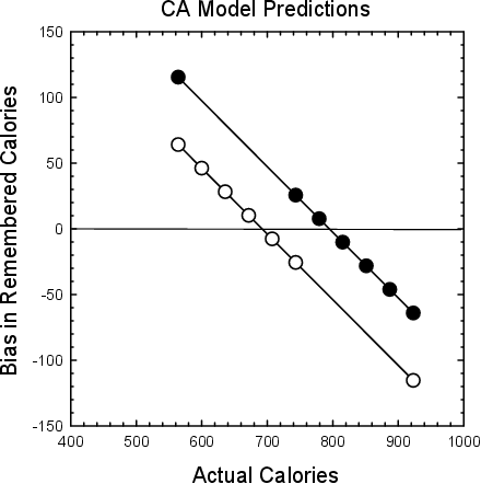
Figure 1: Biases in recall predicted by the CA model for positive skew (open symbols) and negative skew (filled symbols).
In Equation 1, any uncertainty about the stimulus value (indexed by λ less than 1.0) is resolved toward the prototype value. Given that Vik would be the recalled value of stimulus i, the bias would then be:
| Biasik = Vik − Si (2) |
So, if the recalled value (Vik) is greater than Si, then there is a positive bias or overestimation of the value; and if it is less than Si, there is negative bias or underestimation. Essentially, this equation predicts that all values will be displaced toward the category prototype except the prototype. Thus, the X-intercept for the bias function, i.e. the value for which bias is zero, is the inferred to be the value of the prototype.
To understand why this strategy improves average accuracy, consider the case of an observer who has no knowledge of the actual stimulus value. In this case, the best guess will be the mean of the category, because that will be the value that would minimize the mean squared error of estimates. By similar reasoning, if an observer cannot remember the exact stimulus value such that the observer’s best guess would be normally distributed around the actual stimulus value (best-guess distribution), then average accuracy can be improved by picking a value in that best-guess distribution that is closer to the mean of the larger distribution from which the stimulus was sampled. On average, this strategy will improve average accuracy — reduce mean squared error of estimates — because these guesses will on average be closer to other values in the distribution.
In the case of symmetric distributions, such as bell-shaped distributions with many items at the mean and fewer towards the tails, uniform distributions with equal numbers of items at all locations, or u-shaped distributions with fewer items at the mean and many towards the tails, the central tendency of the category as measured by either the mean or median will be exactly at the center of the range of values. According to Equations 1 and 2, recall will then be biased towards the center of the range. In the case of skewed distributions, both the mean and median will be higher for values sampled from negatively-skewed distributions than from positively-skewed distributions. Following Equations 1 and 2, recall will then be biased upward for a negatively skewed distribution and downward for a positively skewed distribution.
Figure 2: Top panel demonstrates differences in evaluation predicted by RF Theory for positive skew (open symbols) and negative skew (filled symbols). Bottom panel demonstrates biases in recall predicted by the modified RF model. 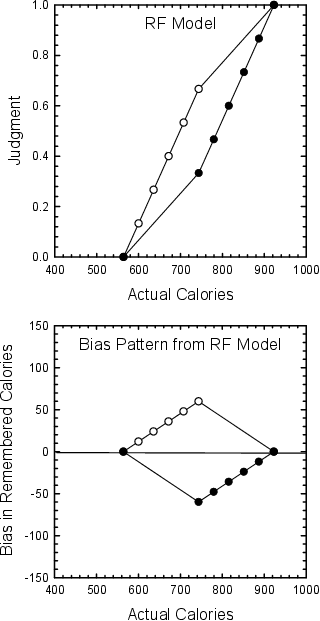
To see how these biases would affect recall of values in skewed distributions, consider the pattern of biases presented in Figure 1 (compare to Figure 2 bottom panel, which presents the predictions of the modified range-frequency model, and Figure 4, which presents the predictions of the comparison-induced distortion model). Figure 1 demonstrates the biases predicted by the CA model for the negatively- and positively-skewed distributions used in Experiments 1 and 2 (described shortly; this graph assumes that the value of Parameter λ in Equation 1 is 0.5). Notice that all of the values sampled from the negatively skewed distribution presented as filled circles — including the smallest and largest values — are above the corresponding values sampled from the positively skewed distribution presented as open circles. In essence, the CA model predicts that the shifting of the distribution mean results in a corresponding shift in the X-intercept of the bias functions, as the X-intercept represent the distribution mean, which is higher for the negatively skewed set.
Duffy, Huttenlocher, Hedges, and Crawford (2010) tested this prediction in a psychophysical experiment in which participants reproduced line lengths drawn from a negatively or positively skewed distribution. Lines appeared briefly for 1 s and then, after a 1 s delay, an anchor line appeared on the screen that participants adjusted to the size of the presented line. The pattern of bias they observed was close to that shown in Figure 1, with both bias functions fairly linear, negatively sloped, and with X-intercepts close to the means of the distributions. Consistent with the CA model, the results did not show greater differences between values within the dense regions relative to sparse regions of the distribution. Applied to the stimuli used in Experiments 1 and 2, the CA model along with the Duffy et al. results would suggest that consumers may have notions about the average caloric values of hamburgers and adjust toward these values in recall, biasing memory of caloric values upwards or downwards for the negatively skewed distribution than for the positively skewed distribution, without producing greater differences between values within the dense regions relative to sparse regions. The uniform bias effect of context on different stimulus values is due to the stimulus distribution being characterized by a single parameter, the mean, and hence density within a region is not represented. Note that this finding is at odds with patterns of results found for category rating measures of evaluation.
When might density effects emerge in memory for stimulus values? Wedell (1996) demonstrated that, when memory constraints were minimal, participants could access the context free stimulus representation, and similarity judgments did not reflect density effects. However, when memory was taxed, large density effects emerged. Similarly, Pettibone and Wedell (2007a) demonstrated that categorical bias in ratings did not emerge when the stimulus was present, but large effects did emerge when the names of the stimuli were learned and then names served as cues for subsequent rating. This type of situation in which values are recalled from name or label cues is common in everyday life. Returning to previous examples, one may be given the cue “the second apartment seen” and then have to reproduce information about the size of its rooms. The present research then was designed to test the boundary conditions for the findings of Duffy et al. (2010) by having participants learn attribute values for labeled stimuli, and then having them reproduce those values from label cues after a short delay. These conditions are particularly common for consumers choosing between products where they know the names of the products and they need to recall the product attribute values to make a decision. Under these circumstances, we would expect density effects to emerge and produce a pattern of bias quite different from that predicted by the CA model and shown in Figure 1.
We next present two models that predict density effects on recall of attribute values under these circumstances: a modification of the range-frequency model (Wedell, 1996) and the comparison-induced distortion model (Choplin & Hummel, 2002).
Previous models of distribution-density effects were primarily designed to explain judgments on category-rating measures of evaluation (but see Corter, 1987; Krumhansl, 1978; Schifferstein & Frijters, 1992; Wedell, 1996; for exceptions). Parducci’s (1965; 1995) Range-Frequency (RF) theory is, perhaps, the most successful model of contextual evaluation (especially under the conditions explored in Experiments 1 and 2 in which all values were presented simultaneously; Parducci, 1992). The top panel of Figure 2 demonstrates the pattern of category rating judgments predicted by RF theory if participants were to evaluate the values sampled from the negatively and positively skewed distributions used in Experiments 1 and 2 (this graph assumes equal weighting of range and frequency principles).
Whereas the CA model predicts that values sampled from negatively-skewed distributions will be recalled larger than values sampled from positively-skewed distributions (see Figure 1), RF theory predicts that category-rating evaluations of values sampled from positively-skewed distributions will be evaluated larger than values sampled from negatively-skewed distributions. Furthermore, in contrast with the CA model, which predicts that all differences will be undervalued, RF theory predicts that differences in dense regions will be overvalued relative to differences in sparse regions. Finally, whereas the CA model predicts that recalled values will be a linear function of presented values, albeit with a less steep slope, RF theory predicts negatively accelerated functions (curving downward) for positively skewed distributions and positively accelerated functions (curving upward) for negatively skewed distributions.
Parducci’s (1965; 1995) RF theory explains why consumers judge values drawn from positively skewed distributions to be larger than values drawn from negatively skewed distributions and also why they overweight differences in dense regions relative to differences in sparse regions, by assuming that they use frequency (i.e., percentile rank) information in evaluation (e.g., an item at the 95th percentile would have a value higher than 95\% and lower than only 5\% of the other values in the distribution; see Stewart, Chater & Brown, 2006, for an application of this model to loss aversion). According to this theory, consumers judge values drawn from positively skewed distributions (top curve, open symbols in the top panel of Figure 2) to be larger than values drawn from negatively skewed distributions (bottom curve, filled symbols in the top panel of Figure 2), because percentile ranks accrue rapidly at the lower end of positively skewed distributions but accrue very slowly at the lower end of negatively skewed distributions. A value drawn from a positively skewed distribution will then have a higher percentile rank than the same value drawn from a negatively skewed distribution (i.e., in Figure 2, 743.5 calories is at the 83rd percentile in the positively skewed distribution [6 out of 7], but is only at the 17th percentile in the negatively skewed distribution [2 out of 7]).
Furthermore, according to this theory, consumers overweight differences in dense regions relative to differences in sparse regions, because percentile rank differences accrue quicker in dense regions than in sparse regions. In the curve representing evaluations of values drawn from the positively skewed distribution in the top panel of Figure 2 (top curve, open symbols), the difference between the percentile rank of 564.0 calories (0th percentile) and 743.5 calories (83rd percentile) is greater than the difference between the percentile ranks of 743.5 calories and 923.0 calories (100th percentile). Likewise, in curve representing evaluations from the negatively skewed distribution in the top panel of Figure 2 (bottom curve, filled symbols), the difference between the percentile ranks of 743.5 calories (17th percentile) and 923.0 calories (100th percentile) is greater than the difference between the percentile rank of 564.0 calories (0th percentile) and 743.5 calories (see Birnbaum, 1974, and Niedrich et al., 2000, for strong tests of the range-frequency model predictions of density effects).
Formally, the RF model predicts that the internal judgment of stimulus i in context k on a 0–1 scale is a weighted average of two proportions, the range value, Rik, and the frequency value (i.e., proportional rank), Fik:
| Jik = w Rik + (1−w) Fik (3) |
where w is the relative weighting of range values. The range value is calculated by the proportion of the range falling below the stimulus value and the frequency value is calculated by the proportion of ranks falling below the stimulus rank (i.e., the percentile rank divided by 100). When the end-stimuli are equated across distributions, one typically assumes that range values for the same stimuli will be equated as well. Thus, all contextual effects in this case are due to the different frequency values. Percentile ranks rise quickly in the positively skewed distribution so that the judgment of a mid-range stimulus will be above the midpoint of the scale. Alternatively, percentile ranks rise slowly in the negatively skewed distribution so that the judgment of a mid-range stimulus will be below the midpoint of the scale. This bias is in the opposite direction as predicted by the CA model and is nonlinear so that effects are minimized at the end stimuli.
Note that because RF theory applies to evaluation and not to recall of stimulus information, it does not make direct predictions concerning how memory for stimulus values will be altered by the density manipulation. To do so requires some auxiliary assumptions. Following Higgins and Lurie (1983), we may assume that evaluations may be better remembered than the stimulus values themselves when the delay between encoding and recall is sufficiently long. Higgins and Lurie found that when asked to recall values after a long delay, participants responded as if they mapped their previous category ratings onto the currently available contextual set of stimulus values. In line with this finding, we assume that implicit RF values that may been generated at encoding are then mapped onto the remembered range or mean of values in memory.
Equation 4 presents a flexible approach to consider how RF values may be mapped onto the response scale:
| Biasik = c + a µk + b | ⎡ ⎢ ⎣ | w |
| + (1−w) Fik | ⎤ ⎥ ⎦ | − Si (4) |
where Si is the stimulus value and w is the relative range weighting. If we wish to consider a simple linear transformation that does not depend on distribution, then we would use the parameters c and b only and set a to 0. When this is done, c is the response value assigned to the minimum judgment value (0) and b is a multiplicative constant relating changes in judgment values to changes on the response scale. The pattern of bias predicted by the RF model of Equation 4 is illustrated in the bottom panel of Figure 2, with w = .5 and assuming a simple matching transformation with c = 564 (the minimum value presented) and b = 923−564 (the range of values presented). All differences in bias between the two distributions are due to the RF model, with no differences predicted at the end stimuli, since these have the same range and frequency values across the two distributions. The key point here is that the predicted bias from a model based on RF values is very different from that based on the CA model. Whereas the CA model predicts linear functions, the RF model predicts nonlinear functions. Whereas the CA model predicts the negatively skewed function is above the positively skewed function, the RF model predicts the reverse. Thus, the predictions from these two models should be easily distinguishable. RF theory predicts that for positively skewed distributions there will be larger differences between the recalled values of attributes at the lower end of the range than at the upper end of the range. That is, when trying to recall the values 564.0, 743.5, and 923.0 calories, there will be biases such that the difference between the recalled values of the lower two will be greater than the difference between the recalled values of the upper two. This pattern will be reversed for the negatively skewed distribution, such that the difference between the recalled values of the lower two will be smaller than the difference between the recalled values of the upper two.
It is also useful to consider how the RF and CA models might be combined to produce a more complex pattern of bias. This is captured in Equation 4 by the inclusion of a term weighting the mean of the relevant distribution, a µk. As a grows larger, responses shift more toward the mean of the distribution, as postulated by the CA model. In terms of the bottom panel of Figure 2, this means the bias function for the positive skewing condition would shift down relative that for the negative skewing condition. This results in responses to the end stimuli showing assimilation while responses for the middle stimuli still show contrast. In Section 4, we fit a three-parameter version of Equation 4 (with a, b and w free to vary) as well as a four-parameter version (with c additionally free to vary).
In addition to range-frequency theory, a host of other models have been proposed to explain particular aspects of contextual effects on category ratings (Baird, 1997; Haubensak, 1992; Stewart & Brown, 2004; Stewart et al., 2006; Petrov & Anderson, 2005). Like RF theory, these approaches generally do not address both evaluation and estimation from memory. An alternative theory that predicts density effects both on memory estimation and evaluation is the comparison-induced distortion theory (CID) developed by Choplin and her colleagues (Choplin, 2007; Choplin & Hummel, 2002). Thus, CID theory may serve as a link to understanding how context affects both judgment and memory and is discussed next.
Choplin and her colleagues have proposed an alternative account of distribution-density effects (called comparison-induced distortion theory or CID theory; see Choplin & Hummel, 2002, 2005, for a discussion of these effects and Choplin, 2007, for mathematical modeling of these effects). The research reported here is the first to investigate these predictions empirically for recall of attribute values. At encoding participants might look at a list of hamburgers and their associated calories and compare the numbers of calories associated with hamburgers. Later when participants are trying to recall the number of calories in hamburgers, they might remember the comparative judgments (e.g., more calories than the ¼ lb. Burger) even if they have forgotten the exact values associated with the hamburgers and rely on that comparative judgment to produce an answer (Higgins & Lurie, 1983).
The basic idea underlying this account is that by having only inexact memory for some of the values, knowing the rank order, and interpolating intermediate differences between values to fill in the memory gaps as best possible, consumers will inevitably overestimate differences between values in the dense regions and underestimate differences in the sparse regions of attribute space. This interpolation of intermediate differences between values could be limited to adjacent items, but would not need to be. Indeed mathematical modeling reported on in Section 4 found that the model fit better when each value was equally likely to serve as a comparison stimulus to all of the other values.
According to the CID theory view, consumers interpolate intermediate differences between values because language-expressible magnitude comparisons (e.g., “this hamburger has more calories than that hamburger”) suggest intermediate differences (Choplin & Hummel, 2002). The judgment that a hamburger contains “more calories than the ¼ lb. Burger”, for example, would suggest that it is unlikely to have 1 more calorie than the ¼ lb. Burger. Although one more calorie is technically “more”, a difference of 1 calorie is less than consumers typically mean when they make such comparative judgments. If there were only a 1 calorie difference, most native English speakers would have judged the two hamburgers to have “approximately the same” number of calories. The hamburger would also be unlikely to be 1,000 more calories, because 1,000-calorie differences among hamburgers are rare. Rather the comparison “more calories than the ¼ lb. Burger” is likely to suggest an intermediate difference (Rusiecki, 1985). This intermediate difference is called the comparison-suggested difference (D), because it is the difference that is suggested by the verbal comparison. This difference of D can then be used to interpolate differences and reconstruct unknown values, albeit with systematic biases.
These intermediate-sized D-values may come from a Bayesian estimation process similar to the one used in Huttenlocher and her colleagues’ CA model. For known categories, the primary difference between the CA model and CID may be the category from which the mean is calculated. For the CA model, the relevant category is the entire category. If the to-be-remembered attribute value is the number of calories and the only thing the estimator knows about the item being estimated is that it is a hamburger, then the relevant category will be all known hamburgers. However, if consumers also know that the to-be-estimated hamburger has “more calories than the ¼ lb. Burger”, then the relevant category may not be all known hamburgers, but rather just those that have more calories than the ¼ lb. Burger. Hamburgers that have fewer calories than the ¼ lb. Burger could be excluded from the category, thereby partitioning the category into two categories: those with more and those with fewer than the ¼ lb. Burger. The mean of the category of hamburgers with more calories than the ¼ lb. Burger will be greater than the mean of the entire, unpartitioned category. Therefore, the CID theory may be a variation of the CA model under specific conditions (but see Choplin & Hummel, 2005, for a demonstration of CID effects in a novel category where CID theory cannot be considered a variation of the CA model).
No matter where these intermediate-sized D-values come from (D was a free parameter in the modeling presented below), consumers might rely upon them to interpolate differences and reconstruct values from memory whenever their memories are inexact. In particular, the comparison-biased recalled value of item i when compared to item j (Vij) might be a weighted average of the poorly remembered, but unbiased, stimulus value of i (Si) and the expected value that is created by the comparison (Eij; E for expected) where the expected value of item i can be calculated from the poorly remembered, but unbiased, value of the stimulus, item j, to which item i is compared (Sj) and the comparison-suggested difference (D):
|
Here v represents the weight given to the poorly remembered, but unbiased, stimulus value of i (Si) bound between 0 and 1.
Figure 3: Predicted comparison-biased recall of values from memory. Arrows represent predicted biases in values drawn from positively and negatively skewed distributions. CID predicts that the 564.0-calorie and 923.0-calorie hamburgers will be recalled smaller in the positively skewed distribution and larger in the negatively skewed distribution, while the 743.5-calorie hamburger will be recalled larger in the positively skewed distribution and smaller in the negatively skewed distribution. 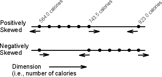
This model predicts that recall of values that are closer to each other than D will be biased apart and recall of values that are farther from each other than D will be biased together. The exact predicted biases will depend upon the comparison-suggested difference (D). The Bias of stimulus i when compared to stimulus j then can be calculated as the difference between the recalled value (Vij) and the stimulus value (Si).
| Biasij = Vij − Si (6) |
A value that is compared to a value that is slightly lower than it (i.e., where the difference is less than D), for example, will then be biased upwards, because Eij will be greater than Si (since Sj + D > Si given that D > Si − Sj) producing a positive bias.
Figure 3 presents a schematic representation of how the CID model might apply to the stimulus design of Experiments 1 and 2, assuming that D is larger than the smallest presented differences and smaller than the largest presented differences. Because values in the dense regions would be biased apart relative to values in sparse regions, CID predicts that differences in dense regions will be overvalued relative to differences in sparse regions. Values in the dense regions (i.e., 564.0 and 743.5 calories in the positively skewed distribution and 743.5 and 923.0 calories in the negatively skewed distribution) will be biased away from adjacent values. The recalled values of the 564.0-calorie hamburger in the positively skewed distribution and the 743.5-calorie hamburger in the negatively skewed distribution will be biased downwards (represented by the leftward arrows in Figure 3); and the recalled values of the 743.5-calorie hamburger in the positively skewed distribution and the 923.0-calorie hamburger in the negatively skewed distribution will be biased upwards (represented by the rightward arrows in Figure 3). This pattern is reversed for the positively skewed distribution.
Similar to the CA model, if D were extremely small, then all values would be biased together (assimilation). However, the CID model predictions in this case differ from the CA model prediction as the degree to which the values would be biased together would be greater in sparse regions than the dense regions. Hence, rather than the straight-line bias functions shown in Figure 1 for the CA model, the CID model would again have nonlinear functions but the functions would not cross over as all data points would reflect assimilation.
To illustrate the predictions of the CID model, one must make assumptions concerning how the retrieved comparison stimulus depends on context. A simplifying assumption is that all values in the distribution are equally likely to serve as a comparsion stimulus. Thus, bias for stimulus i in context k can be represented as follows:
| Biasik = v Si + (7) |
| (1−v)[∑(SAj − DA) + ∑(SBj+DB)]/6 −Si . |
Figure 4: Biases in recall predicted by the CID model for positive skew (open symbols) and negative skew (filled symbols). 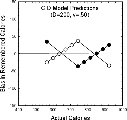
Analogous to the CID model fitting done by Choplin and Hummel (2005), separate D values for upward and downward comparisons are posited. In Equation 7, 1−v is the weighting of the comparison distorted value, Si is the value of the stimulus, SAj is the value of each comparison stimulus above the target value (A for above), DA is the expected difference for each stimulus that is above the target value (note that since these stimuli are above the target the expected difference will be below these stimuli, back down towards the target), SBj is the value of each comparison stimulus below the target value (B for Below), DB is the expected difference for each stimulus that is below the target value (note that since these stimuli are below the target the expected difference will be above these stimuli, back up towards the target), and 6 is the number of comparisons. Equation 7 has three fitted parameters, v, DA and DB.
Figure 4 illustrates the application of this model to the example used for Figures 1 and 2, with DA = DB = 200 and v = 0.5. As shown, the form of the bias functions are essentially the same as described by the modified RF model. However, this version of the model entails a crossing over of the functions so that bias is in the opposite direction for end stimuli than for stimuli in the middle. Both the modified RF model and the standard CID model predict density effects that are qualitatively different from the standard CA model. The goal of Experiments 1 and 2 was to investigate whether recall of values from skewed distributions when memory is taxed and consumers have labels for the to-be-recalled values will follow the pattern described by the CA model or the patterns described by the modified RF and CID models. Results are presented along with the quantitative fits of these models to the data.
Table 1: Presented distributions of hamburgers and associated calories in Experiments 1 and 2.
Experiment 1 investigated distribution-density effects on recall of values from memory when values were presented simultaneously (Haubensak, 1992; Parducci, 1992). Like previous research with numerical stimuli (Birnbaum, 1974; Wedell, Parducci & Roman, 1989), values were presented in ascending or descending orders on the page. Participants viewed either the hamburgers and associated calories listed under positive skew or the ones listed under negative skew in Table 1 and later, after a short distracter task, recalled those values from memory. The CA and CID models predict that the smallest value (564.0 calorie; ¼ lb. Burger) and largest value (923.0 calorie; 2/3 lb. Monster Double Burger) will both be recalled larger if drawn from a negatively skewed distribution than if drawn from a positively skewed distribution. The CID and modified RF model predict that the medium-sized value (743.5 calorie; ½ lb. Big Double Burger) will be recalled larger in the positively skewed distribution than in the negatively skewed distribution.
One hundred people volunteered to participate after being approached by the experimenter on the DePaul University campus or in the surrounding community. Fifty participants were in each of the positively and negatively skewed conditions.
Participants viewed seven hamburgers and their respective caloric values listed vertically from the top of the page to the bottom in either an ascending or a descending order. The hamburgers and their associated caloric values are shown in Table 1. We were primarily interested in recall of three values: the ¼ lb. Burger, ½ lb. Big Double Burger, and 2/3 lb. Monster Double Burger. To create a positively skewed distribution of values, four hamburgers with caloric values between the caloric values of the ¼ lb. Burger and the ½ lb. Big Double Burger were included in the distribution of values (see Table 1). To create a negatively skewed distribution of values, four hamburgers with caloric values between the caloric values of the ½ lb. Big Double Burger and the 2/3 lb. Monster Double Burger were included in the distribution of values.
To ensure that participants spent some time processing the seven values, they were asked whether they were surprised by the number of calories in the distribution of hamburgers they had seen. Participants were then given a distracter task that lasted for approximately one minute in which they reviewed “Things You May Not Know” such as “The 57 on Heinz ketchup bottle represents the varieties of pickle the company once had” and “40\% of McDonald’s profits come from the sales of Happy Meals” and then indicated whether or not they knew these things. This distracter task was followed by a surprise recall task in which they recalled the number of calories in each of the seven hamburgers. The questionnaire on which participants recalled calories presented hamburgers in the same order as the hamburgers were originally presented. Participants were instructed to estimate values, if they could not recall exact values.
Figure 5: Biases observed in Experiment 1 for positive skew (open symbols) and negative skew (filled symbols). 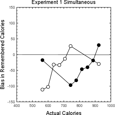
Table 2: Recalled number of calories.
Experiment 1 1/4 lb. Burger 1/3 lb. Cheeseburger 1/3 lb. Bacon Cheeseburger 1/3 lb. Deluxe Burger 1/3 lb. Double Burger 1/2 lb. Big Double Burger 2/3 lb. Big Bacon Double Burger 2/3 lb. Big Bacon Double Deluxe Burger 2/3 lb. Super Bacon Double Burger 2/3 lb. Super Big Bacon Double Deluxe Burger 2/3 lb. Monster Double Burger Experiment 2: Simultaneous presentation 1/4 lb. Burger 1/3 lb. Cheeseburger 1/3 lb. Bacon Cheeseburger 1/3 lb. Deluxe Burger 1/3 lb. Double Burger 1/2 lb. Big Double Burger 2/3 lb. Big Bacon Double Burger 2/3 lb. Big Bacon Double Deluxe Burger 2/3 lb. Super Bacon Double Burger 2/3 lb. Super Big Bacon Double Deluxe Burger 2/3 lb. Monster Double Burger Experiment 2: Sequential presentation 1/4 lb. Burger 1/3 lb. Cheeseburger 1/3 lb. Bacon Cheeseburger 1/3 lb. Deluxe Burger 1/3 lb. Double Burger 1/2 lb. Big Double Burger 2/3 lb. Big Bacon Double Burger 2/3 lb. Big Bacon Double Deluxe Burger 2/3 lb. Super Bacon Double Burger 2/3 lb. Super Big Bacon Double Deluxe Burger 2/3 lb. Monster Double Burger Note: The smallest (1/4 lb. Burger) and largest (2/3 lb. Monster Double Burger) values were recalled larger, but the value at the middle of the range (1/2 lb. Big Double Burger) was recalled smaller, when drawn from the negatively skewed distribution than when drawn from the positively skewed distribution.
Recalled numbers of calories are presented in the top panel of Table 2, with Figure 5 showing the pattern of bias. Consistent with the predictions of the CA model and CID, but not predicted by the modified RF model, the smallest and largest values were recalled significantly larger when they were placed within the negatively skewed distribution than when they were placed within the positively skewed distribution. Participants recalled significantly more calories in the 564.0-calorie ¼ lb. Burger when it was placed in a negatively skewed distribution of values (546.4 calories) than when it was placed in a positively skewed distribution of values (452.9 calories), t(98)=3.47, p < .01. Participants also recalled marginally more calories in the 923.0-calorie 2/3 lb. Monster Double Burger when it was placed in a negatively skewed distribution of values (953.1 calories) than when it was placed in a positively skewed distribution of values (893.3 calories), t(98)=1.79, p < .1.
Consistent with the CID and the modified RF models, but inconsistent with the CA model, participants recalled more calories in the 743.5-calorie ½ lb. Big Double Burger when it was placed in a positively skewed distribution of values (770.5 calories) than when it was placed in a negatively skewed distribution of values (646.5 calories), t(98)=4.64, p < .01. As described earlier, only the CID model predicts this pattern of observed bias for both the end values and the middle value.
The results of Experiment 1 supported the predictions of the CID model. However, the sequences in which values were presented might have made this pattern of results particularly likely. In particular, caloric values were presented simultaneously in either an ascending or a descending order in Experiment 1. This format might have constrained participants to make primarily pairwise comparisons among adjacent values. However, the CID model’s qualitative predictions outlined above do not depend upon values being compared to any particular values (see the model fitting below which found that target values are equally likely to be compared to all contextual values). Furthermore, menus that present nutritional information such as the caloric content of foods often do not present this information in ascending or descending order. The purpose of Experiment 2 then was to investigate whether the effects observed in Experiment 1 would generalize to random sequences of values (Sokolov, Pavlova & Ehrenstein, 2000). Values were presented in random orders either sequentially or simultaneously (Haubensak, 1992; Parducci, 1992).
Two hundred volunteers participated after being approached by the experimenter on the DePaul University campus. There were fifty participants in the negatively skewed condition and fifty participants in the positively skewed condition in each of the simultaneous-presentation and sequential-presentation conditions.
Figure 6: Biases observed in Experiment 2 when values were presented simultaneously (top panel) and when values were presented sequentially (bottom panel) for positive skew (open symbols) and negative skew (filled symbols). 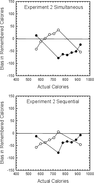
Fifty random sequences were created for each of the positively and negatively skewed distributions of values presented in Table 1. Participants in the simultaneous-presentation condition viewed these seven values presented in a random order from the top to the bottom of the same page. Participants in the sequential-presentation condition saw the exact same 50 sequences as did the participants in the simultaneous-presentation condition, but each of the seven values was presented on a separate page. To ensure that participants spent some time processing these values, they judged whether the numbers of calories in the set of hamburgers they had seen were surprising. Participants then completed the distracter task used in Experiment 1, before they recalled calories. The recall sheet had seven unlabeled blank slots in which participants wrote down the calories of the hamburgers they had seen in the order in which they had seen them. Participants were instructed to estimate, if they could not recall exact values.
The middle and bottom panes of Table 2 present the mean recalled numbers of calories, and Figure 6 presents the mean bias for each stimulus. Consistent with the predictions of the CA model and the CID model, the smallest and largest values recalled for the negatively skewed distribution were significantly larger than were the smallest and largest values recalled for the positively skewed distribution. A 2(skew: positive or negative) x 2(presentation method: simultaneous or sequential) between-subjects analysis of variance (ANOVA) conducted on the lowest calorie hamburger found that the recalled value for the negatively skewed distribution (563.9 calories) was larger than the recalled value for the positively skewed distribution (513.8 calories; actual smallest value was 564 calories), F(1,196)= 14.66, p < .01 (this effect held for both simultaneous, t(98) = 2.86, p <.01, and sequential presentation, t(98) = 2.55, p <.05). There was no effect of the type of presentation on the recall of the smallest value, F(1,196)=2.38, p > .05, nor an interaction, F(1,196) = 0.16, p > .05. A parallel ANOVA was conducted on the highest calorie hamburger, with the recalled value in the negatively-skewed distribution (906.7 calories) also larger than the recalled value in the positively-skewed distribution (872.5 calories; actual largest number was 923 calories), F(1,196) = 9.58, p < .01 (this effect held for both simultaneous, t(98) = 2.05, p < .05, and sequential presentation, t(98) = 2.32, p < .05). Again, there was no effect of the type of presentation, F(1,196)= 1.16, p > .05, nor was there an interaction, F(1,196)= 0.14, p > .05. The results for these two values — the smallest and largest values in these distributions — are consistent with both the CA and the CID models and not predicted by the modified RF model.
Finally, a parallel ANOVA was conducted on the middle-valued target, 743.5 calorie ½ lb. Big Double Burger. Consistent with CID and the modified RF model, but inconsistent with CA, participants recalled more calories when it was placed in a positively skewed distribution of values than when it was placed in a negatively skewed distribution of values, F(1,196) = 71.56, p < .01. This effect was observed both in the simultaneous-presentation condition (t(98) = 6.97, p < .01) and in the sequential-presentation condition (t(98)=5.03, p < .01). There was no effect of the type of presentation, F(1,196)= 1.70, p>.05, nor was there an interaction, F(1,196)= 1.54, p>.05. Only the CID model was able to account for the qualitative biases observed for both the end values and the middle values.
In this section we discuss the model fits to the data illustrated in Figures 5 and 6. Each of these conditions (i.e., Experiment 1, Experiment 2: Simultaneous Presentation, and Experiment 2: Sequential Presentation) has 14 data points (7 values from the positive skew and 7 from the negative skew), making for a total of 52 data points being modeled. Each model was fit using nonlinear iterative regression with a least squares error term. Parameters were free to vary across the three conditions so as to maximize fit. Thus, if a three-parameter model was being fit (i.e., both the modified RF model and the CID model were fit with 3 parameters first), the effective number of parameters was 9, as the three parameters were fit to each condition. The R2 values reported are based on the fit to the full set of 52 data points.
Table 3: Model fit statistics.
Model Condition Parameter values R2 RF-3p Experiment 1 a = .66, b = 418, w = .31 Experiment 2 simultaneous a = .75, b = 314, w = .01 Experiment 2 sequential a = .71, b = 359, w = .39 0.846 RF-4p Experiment 1 c = −19, a = .69, b = 418, w = .29 Experiment 2 simultaneous c = 315, a = .32, b = 324, w = .30 Experiment 2 Sequential c = 227, a = .40, b = 366, w = .57 0.924 CID-3p Experiment 1 v = .564, DA = 333, DB = 190 Experiment 2 simultaneous v = .621, DA= 244, DB = 140 Experiment 2 sequential v = .357, DA = 313, DB = 127 0.805 CID-4p Experiment 1 aPOS = −20,v = .564, DA = 330, DB= 192 Experiment 2 simultaneous aPOS = 249,v = .621, DA = 257, DB = 107 Experiment 2 sequential aPOS = 9, v = .357, DA = 315, DB= 125 0.924 Note: Parameter values specified in Equations 3 through 7, RF = Range-frequency, CID = Comparison Induced Distortion, 3p = three parameters, and 4p = four parameters.
The empirical bias patterns of Figures 5 and 6 do not resemble those predicted by the CA model and shown in Figure 1. When the weighting parameter of the CA model was constrained to be between 0 and 1 and the category prototype was constrained to be higher for the negatively skewed distribution than for the positively-skewed distribution, the CA model was unable to fit the data, with an effective R2 = 0. This is because the data do not show the negatively sloping bias function nor bias functions that are higher for negative than positive skewing. Thus, although the CA model does a good job modeling remembered values when delay between encoding and retrieval is quite short (Duffy et al., 2010), it does not appear capable of explaining the pattern of data obtained in our experiments that utilized a longer forgetting period and label cues.
Two versions of the modified RF model of Equation 4 were fit to the data. The three parameter version fixed c at 0 so that a accounts for any assimilative effects at the end stimuli and w accounts for the basic pattern of data and contrast effects for middle stimuli. This model resulted in a good fit to the data, R2 = 0.846 for this 9-parameter model. The fit of this model is shown in the solid lines of Figure 7 and the parameter values are shown in Table 3. As seen in Figure 7, the model captures the general pattern of the data quite well. The three-parameter range frequency model fits the assimilative effects at the end-points by weighting the means of the distributions and fits the contrastive effects for the middle stimuli by the weighting of frequency values. This model constrains the intercepts to be a function of distribution means. To determine how much of the misfit is due to this constraint, the global intercept parameter, c, was then allowed to vary. This model 12-parameter model fit significantly better than the 9-parameter, R2 = .924 and provided a very good fit to the data.
Figure 7: Fits of the three-parameter CID and the three-parameter modified RF models to the results of Experiments 1 and 2 for positive skew (open symbols) and negative skew (filled symbols). 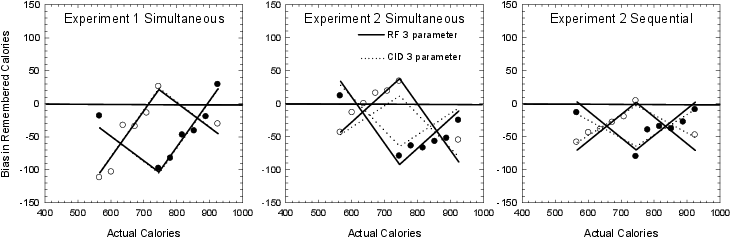
In situations in which delay is short, one might posit the most recent stimulus constitutes the comparison stimuli (Choplin & Lombardi, 2010). In this way, the CID model can generate sequential effects. However, for the current experimental design, there is no reason to posit sequential effects. One might argue that on any given trial each of the other stimuli is likely to serve as a comparison stimulus, as assumed in Equation 7. Alternatively, one might argue that similarity to the target might mediate recruitment of the comparison stimulus. Preliminary modeling that tested between these two possibilities supported the former, and so the model of Equation 7 was fit. This model also did a good job of approximating the data, R2 = .805, 9-parameter fit. The fit of this model is shown as dotted lines in Figure 7 and parameter values are presented in Table 3. Again, the model does a good job capturing the qualitative pattern of the data. Both the three-parameter RF and CID models provide a very close fit to the data of Experiment 1 (left panel of Figure 7). The three-parameter RF model predicts the data from the simultaneous-presentation condition of Experiment 2 better than the three-parameter CID model (middle panel of Figure 7), but the reverse is true for the sequential-presentation condition of Experiment 2 (right panel Figure 7). The three-parameter CID model constrains the extent of the contrast effect by the extent of the assimilation effect. To determine how much of the misfit is due to this constraint, an additive constant was included in Equation 7 for the positive skewing condition, apos. This 12-parameter model is structurally equivalent to the 12-parameter modified RF model and thus provides an identical fit, R2 = 0.924. The fit statistics are shown in Table 3.
In summary, model fitting confirmed that the CA model cannot explain this pattern of data and that the modified RF and CID models provide good quantitative fits to the data with three parameters free to vary for each of the three conditions represented by Figures 4, 5, and 6. The modified RF model fits the form of the bias functions by assuming that values reflect ranks as described by the frequency principle of judgment. It fits the assimilative effects on the end stimuli by adopting an anchoring and adjustment process similar to the CA model that anchors on the distribution means but adjusts in proportion to RF value differences. The CID model fits both assimilation for the end stimuli and contrast for the middle stimuli using a common mechanism, a comparison that is distorted toward the expected difference. Model fitting demonstrated that when a fourth parameter is added to the models, the two models can become equivalent. Because the CID model entails the two effects, its explanatory power is somewhat greater when parameters are constrained.
Two experiments found patterns of recall that were consistent with the predictions of the modified RF model and with the predictions of the CID model, but that were inconsistent with the CA model. In Experiment 1, hamburgers and their associated caloric values were presented simultaneously in either an ascending or a descending order. In Experiment 2, hamburgers and their associated caloric values were presented in random orders wherein the seven hamburgers were presented either simultaneously on the same page or sequentially on seven separate pages. After they were given a distracter task, participants recalled these values from memory using the hamburger labels as retrieval cues.
Both the modified RF model and the CID model fit the data equally well, but the CID model has the advantage that it entails the qualitative finding that the smallest and largest values recalled for the negatively skewed distribution were significantly larger than were the smallest and largest values recalled for the positively skewed distribution. Furthermore, other extant models of density effects on evaluation typically are not designed to predict density effects on recall (i.e., Baird, 1997; Haubensak, 1992; Stewart & Brown, 2004; Stewart et al., 2006; Petrov & Anderson, 2005), making the predictions of the CID model somewhat unique.
The results of Experiments 1 and 2 most likely differed from the results reported by Duffy et al. (2010) because memory was taxed (Wedell, 1996) and participants had associated labels with each of the to-be-recalled attribute values (Pettibone & Wedell, 2007a). Similar memory effects wherein relational information later biases recall have been reported in the stereotype literature (Higgins & Lurie, 1983). In the experiments reported by Duffy et al., there was only a 1 second delay so fine-grain information was likely highly accessible and participants only recalled one item. By contrast, there was a much longer delay in the current experiments and participants recalled seven values. Duffy et al. (2010) also used analog visual stimuli, rather than the numerical stimuli used here. The conditions in the experiments reported here may better reflect many real-life decision-making situations, as home-purchase decisions might depend upon recall of room sizes, automobile-purchase decisions upon recall of mileage, and dietary decisions upon recall of calories and fat content. In such situations, consumers have to make decisions despite a variety of distractions and after a long delay, and they may use labels to recall product attribute values (e.g., the second home we saw, the green car, the ¼ lb. Burger).
Duffy et al. (2010) argued that their results demonstrated that comparisons to preceding values presented in a sequence affected recall of the to-be-judged stimulus only to the extent that the preceding stimulus changed the mean of the category. Language-based pairwise comparisons were not supposed to play a role. It is important to point out that the CID model predicts effects of the preceding stimulus only if and when the to-be-judged stimulus is verbally compared to the preceding stimulus. The paradigm used by Duffy et al. might have made such verbal comparisons unlikely. Other paradigms and real-life situations might make verbal comparisons more likely. More research will be needed before it is possible to conclude that comparisons to preceding values presented affected recall only to the extent that the preceding stimulus changed the mean of the category. Further, the density effects found in the present experiments clearly indicate that distributional information other than the mean (i.e., the relative densities) is affecting recall.
Experiments 1 and 2 used unimodal, positively and negatively skewed distributions. Yet all three of the models presented here — the CA model, the modified RF model, and the CID model — make predictions about recall of values from other distributions such as normal, uniform, and u-shaped distributions. The CA model predicts that recall will be biased towards the means of the relevant category or categories. The modified RF model predicts that recall will reflect percentile rankings such that differences between stimulus values will be greater in dense than in sparse regions. The CID model predicts that pairwise, verbal comparisons between values will tend to bias recall towards more uniform differences between values, pushing memory for values in dense regions towards sparse regions and creating a predictable pattern of assimilation and contrast effects on recall. Future research should investigate effects of factors such as different distributions, the length of the delay, the number of items recalled, the stimuli used (e.g., visual versus numerical stimuli), and whether items are given labels are likely to affect the patterns of bias one observes and further distinguish among these models.
The results presented here have important implications for consumer choice. Much of the research that has studied the effects of density on decision making has presented options to participants and participants make decisions while the options remain in view (e.g., Pettibone & Wedell, 2000; Wedell & Pettibone, 1996). The finding that the smallest and largest values in Experiments 1 and 2 were recalled significantly larger when they were drawn from the negatively-skewed distribution than when they were drawn from the positively-skewed distribution and the fact that this effect was not observed in previous research on attribute evaluation suggests that there could be situations wherein the effects of density on decisions might differ if consumers make decisions while the options remain in view than if consumers make decisions after a delay. Based on the research reported here, we believe that decisions about a host of everyday consumer purchases (food, household items, etc.) may differ when recalling attributes from memory versus when viewing the attribute listing directly. Given the contextual nature of choice, it is also possible that effects like the asymmetric dominance effect (Choplin & Hummel, 2002, 2005) and the phantom decoy effect (Pettibone & Wedell, 2007b) might be stronger after a delay than when the options remain in view. Judgments of body sizes could also differ if items remain in view or are judged from memory (Choplin, 2010) as could other social comparisons (Bloomfield & Choplin 2011; Pettibone & Wedell, 2007a). Future research should pursue these questions to investigate whether judgments and decisions made immediately differ from decisions made after a delay.
The results presented here have specific implications for recent efforts to post nutritional information such as caloric content in restaurants and on menus. Previous research on category rating evaluations would have suggested that menus with positively skewed distributions of caloric content (i.e., menus with many reduced-calorie options and only a few highly caloric options) would lead to portions being judged more caloric, which could have in some circumstances led consumers to be more careful. This pattern of results could have led health promoters to advocate for the adoption of menus with positively skewed distributions of caloric content. The current results suggest that such a policy could very well be effective as the medium-sized, 743.5-calorie 1/2 lb. Big Double Burger was recalled as larger in the positively skewed distribution than in the negatively skewed distribution. However, the current results also suggest a boundary conditions on this generalization as the opposite pattern was observed for the small 564.0-calorie 1/4 lb. Burger and the large 923.0-calorie 2/3 lb. Monster Double Burger. The adoption of such a menu, then, could backfire for extremely small and extremely large items on the menu. Consumers could start eating extraordinary amounts of the reduced-calorie items and could underestimate the harm cause by the most extreme highly caloric options. These effects are likely to be particularly strong as these types of dietary decisions are typically highly reliant on memory. In applying these findings to real-world implications for the design of menus and food presentation, it will be important to clarify the boundary conditions under which these memory effects occur and how they affect actual dietary decisions.
Baird, J. C. (1997). Sensation and judgement: Complementarity theory of psychophysics. Hillsdale, NJ: Lawrence Erlbaum.
Birnbaum, M. H. (1974). Using contextual effects to derive psychophysical scales. Perception & Psychophysics, 15, 89–96.
Bloomfield, A. N. & Choplin, J. M. (2011). I’m “better” than you: Social comparison language produces apparent assimilation and contrast effects. Language and Cognition, 3(1), 15–43.
Choplin, J. M. (2007). Toward a comparison-induced distortion theory of judgment and decision making. In J. A. Elsworth (Ed.), Psychology of decision making in education, behavior and high risk situations (pp. 11-40). Hauppauge, NY: Nova Science.
Choplin, J. M. (2010). I am “fatter” than she is: Language-expressible body-size comparisons bias judgments of body size. Journal of Language and Social Psychology, 29, 55–74.
Choplin, J. M., & Hummel, J. E. (2002). Magnitude comparisons distort mental representations of magnitude. Journal of Experimental Psychology: General, 131(2), 270–286.
Choplin, J. M., & Hummel, J. E. (2005). Comparison-induced decoy effects. Memory & Cognition, 33, 332–343.
Choplin, J. M. & Lombardi, M. M. (2010). Comparison-induced sequence effects. Proceedings of the Thirty-Second Annual Conference of the Cognitive Science Society.
Clifford, S. (2013, June 29). Why Healthy Eaters Fall for Fries. The New York Times. Retrieved from http://www.nytimes.com.
Cooke, A. D. J., & Mellers, B. A. (1998). Multiattribute judgment: Attribute spacing influences single attributes. Journal of Experimental Psychology: Human Perception and Performance, 24, 496–504.
Corter, J. E. (1987). Similarity, confusability, and the density hypothesis. Journal of Experimental Psychology: General, 116, 238–249.
Duffy, S., Huttenlocher, J., Hedges, L. V., & Crawford, L. E. (2010). Category effects on stimulus estimation: Shifting and skewed frequency distributions. Psychonomic Bulletin & Review, 17, 224–230.
Haubensak, G. (1992). The consistency model: A process model for absolute judgments. Journal of Experimental Psychology: Human Perception and Performance, 18, 303–309.
Higgins, E. T., & Lurie, L. (1983). Context, categorization, and recall: The “change-of-standard” effect. Cognitive Psychology, 15, 525–547.
Huttenlocher, J., Hedges, L. V., & Duncan, S. (1991). Categories and particulars: Prototype effects in estimating spatial location. Psychological Review, 98, 352–376.
Huttenlocher, J., Hedges, L. V., & Vevea, J. L. (2000). Why do categories affect stimulus judgment? Journal of Experimental Psychology: General, 129(2), 220–241.
Krumhansl, C. L. (1978). Concerning applicability of geometric models to similarity data: Interrelationship between similarity and spatial density. Psychological Review, 85, 445–463.
Niedrich, R. W., Sharma, S., & Wedell, D. H. (2001). Reference price and price perceptions: A comparison of alternative models. Journal of Consumer Research, 28(3), 339–354.
Parducci, A. (1965). Category judgments: A range-frequency model. Psychological Review, 72, 407–418.
Parducci, A. (1992). Comment on Haubensak’s associative theory of judgment. Journal of Experimental Psychology: Human Perception and Performance, 18, 310–313.
Parducci, A. (1995). Happiness, pleasure and judgment: The contextual theory and its applications. Mahwah, NJ: Lawrence Erlbaum.
Petrov, A. A., & Anderson, J. R. (2005). The dynamics of scaling: A memory-based anchor model of category rating and absolute identification. Psychological Review, 112, 383–416.
Pettibone, J. C., & Wedell, D. H. (2000). Examining models of nondominated decoy effects across judgment and choice. Organizational Behavior and Human Decision Processes, 81, 300–328.
Pettibone, J. C., & Wedell, D. H. (2007a). Of gnomes and leprechauns: The recruitment of recent and categorical contexts in social judgment. Acta Psychologica, 125, 361–389.
Pettibone, J. C., & Wedell, D. H. (2007b). Testing alternative explanations of phantom decoy effects. Journal of Behavioral Decision Making, 20, 323–341.
Rusiecki, J. (1985). Adjectives and Comparison in English. New York: Longman.
Schifferstein, H. N. J., & Frijters, J. E. R. (1992). Contextual and sequential effects on judgments of sweetness intensity. Perception & Psychophysics, 52, 243–255.
Sokolov, A., Pavlova, M., & Ehrenstein, W. H. (2000). Primacy and frequency effects in absolute judgments of visual velocity. Perception & Psychophysics, 62, 998–1007.
Stewart, N., & Brown, G. D. A. (2004). Sequence effects in the categorization of tones varying in frequency. Journal of Experimental Psychology: Learning, Memory, and Cognition, 30, 416–430.
Stewart, N., Chater, N., & Brown, G. D. A. (2006). Decision by sampling. Cognitive Psychology, 53, 1–26.
Volkmann, J. (1951). Scales of judgment and their implications for social psychology. In J. H. Roherer & M. Sherif (Eds.), Social psychology at the crossroads (pp. 279-294). New York: Harper & Row.
Wedell, D. H. (1996). A constructive-associative model of contextual dependence of unidimensional similarity. Journal of Experimental Psychology: Human Perception and Performance, 22, 634–661.
Wedell, D. H., Hicklin, S. K., & Smarandescu, L. O. (2007). Contrasting models of assimilation and contrast. In D. A. Stapel & J. Suls (Eds.), Assimilation and contrast in social psychology (pp. 45–74). New York: Psychology Press.
Wedell, D. H., Parducci, A., & Roman, D. (1989). Student perceptions of fair grading: A range-frequency analysis. American Journal of Psychology, 102, 233–248.
Wedell, D. H., & Pettibone, J. C. (1996). Using judgments to understand decoy effects in choice. Organizational Behavior and Human Decision Processes, 67, 326–344.
Copyright: © 2014. The authors license this article under the terms of the Creative Commons Attribution 3.0 License.
This document was translated from LATEX by HEVEA.