Judgment and Decision Making, Vol. 9, No. 5, September 2014, pp. 387-402
An interpretation of focal point responses as non-additive beliefsAylit Tina Romm* |
This paper provides a novel interpretation of focal point responses (0, 50, 100 percent) in terms of ambiguous beliefs dynamics that arise in new developments of decision theory such as Choquet expected utility theory. In particular, focal point responses that have been updated from nonfocal responses can be interpreted as non-additive beliefs that account for psychological bias. A focal point response of 100 that has been updated from a nonfocal response can be represented by a non-additive belief that has been updated according to the Overestimating Update Rule. A focal point response of zero that has been updated from a nonfocal response can be represented by a non-additive belief that has been updated according to the Underestimating Update Rule. Focal point responses given consistently over time are not subject to psychological bias, and can be represented by additive probability distributions. Estimation results show such a model to be a very good fit to the data.
Keywords: focal point response, Choquet expected utility,
psychological bias, non-additive belief, update rule.
Major life decisions typically rely on agents’ expectations about uncertain events in the future. These expectations, in turn, are formed from subjective beliefs about the probability distributions of such events. In surveys, such subjective probability distributions are often elicited through responses to questions regarding probabilities of particular events. Researchers then use these responses as a measure of true beliefs. Authors such as Bloom et al. (2007) and Romm (2014) look at the effect of survival probabilities and retirement probabilities, respectively, on the wealth accumulation decisions of households.
Concern, however, has been expressed in the literature about the pattern of responses given to such questions (e.g., Hurd & McGarry, 1995; Hurd et al., 1998; and Basset & Lumsdaine, 2001). While general inconsistencies in such answers have been noted, the concentration of answers around focal points (0, 50 and 100 percent) has been of notable concern (see Section 2). While answers clustered at 50 are certainly problematic, focal point answers of 0 and 100 seem much more questionable, in that it is unrealistic for an agent to know with complete certainty whether an uncertain future event will occur or not. Nonfocal point responses are often referred to in the literature as precise answers, implying that focal point responses are imprecise, or inaccurate.
In this paper, some dynamic elements of data from the US Health and Retirement Study (HRS) are used to show that there are two different kinds of focal point responses given close to the time of the event in question—in this case—working past age 62: those that are roughly accurate and those that are not. The paper shows that focal point responses given consistently, over the time the respondent is questioned in the HRS, are quite accurate, whereas focal point responses given only closer to the event in question, which have been updated from nonfocal responses given at younger ages, are too extreme. Thus, what is of interest is the dynamic process that leads the agent to make such focal responses later in time.
While the literature seems to concur that focal point responses of 0 and 100 usually do not indicate certainty, this paper provides a formal decision theoretic approach that explains the dynamics of the agents’ responses. More specifically, a focal point response of 100 or 0 (or 1,0 on a 0–1 scale) that has been updated from a nonfocal response (which for the purposes of this paper is any answer other than 0 and 100) is represented as a neo-additive capacity in the sense of Chateauneuf et al. (2007).
A neo-additive capacity is a non-additive probability that represents a deviation from a probability from a distribution that is additive, a distribution in which the probabilities over the state space sum to one. The deviation expresses ambiguity, or lack of confidence in the additive probability distribution. The deviation could involve over- or underestimation.1 In the present context, when ambiguity increases over time, the agent resolves this ambiguity by expressing complete confidence in the extreme belief that he/she will or will not continue to work full time after age 62.
The formal interpretation presented is consistent with focal point responses nearer age 62 that have been updated from nonfocal answers given at younger ages. In particular, this interpretation is consistent with the data according to which focal point responses given consistently over the time that individuals are questioned are quite accurate, whereas focal point responses given only closer to the event in question (and that have been updated from nonfocal answers) are biased, in the sense that the expressed probability is more extreme than the objective probability.
The contribution of this paper relates both to the data themselves and to their use to make a theoretical contribution. Firstly, I show that, with the exception of married men, the subjective probability of working past age 62 fails to converge to the corresponding objective probability as individuals approach age 62. In particular, there is an upward bias that is non-decreasing over time—an observation that represents an apparent violation of the Rational Bayesian Learning paradigm. The Rational Bayesian Learning paradigm involves the notion that, although individuals need not know at the outset what is going to happen in the future, as time passes and they acquire more experience and knowledge regarding the probability of a future event occurring, their subjective assessment of the relevant probability should converge to the objective probability (defined as the relative frequency of the event occurring for a group of respondents).
Secondly, I find an increased tendency at older ages to give a focal point response of 100 for the probability of working full time after age 62. This phenomenon is the primary cause of the failure of the subjective probability of working past age 62 to converge to the corresponding objective probability over time. It is these initial observations that result in the paper studying focal point responses more closely, culminating in the formal interpretation of such focal point responses within a decision theoretic framework. Thus, while authors such as Hurd and McGarry (1993) and Hurd (2009) have also found a tendency for individuals in the Health and Retirement Study to overestimate the probability of working past age 62, this paper is the first to show the role of focal point responses in explaining this phenomenon.
The paper proceeds as follows. Section 2 briefly reviews the existing literature on focal point answers. Section 3 illustrates the stylized facts in the data. Section 4 provides the theoretical framework used to explain the observations in the data. In Section 5, the relevant parameters for the suggested model are estimated. Section 6 concludes.
While theoretically answers of 0 and 100 should display certainty, the empirical literature thus far tends to agree that focal point answers of 0 and 100 are a reflection of the agent’s uncertainty regarding the relevant probability distribution. According to Lillard and Willis (2001) and Hill et al. (2004), this uncertainty results in agents reporting the modal (most likely) probability in response to subjective probability questions. Basset and Lumsdaine (2001) and Huynh and Jung (2010) show that individuals who give answers of zero and 100 are less educated and have lower income levels than other individuals. This suggests that answers of zero and 100 demonstrates lack of understanding of the question or the concept of a probability. Such agents are, in this sense, uncertain as to how to respond. Willis (2005) shows, using a sample of individuals over 70 from the ahead cohort of the HRS, that individuals who give a focal point response of zero to a question regarding the probability of survival, have actual survival probabilities 13 percentage points higher than those individuals giving a nonfocal response very close to zero. Similarly, those giving a response of 100 to this question have a survival probability 3.8 percentage points lower than individuals giving nonfocal responses very close to 100.
The opinion on answers of 50 is different. While Bruine de Bruin et al. (2000) and Lilard and Willis (2001) say answers of 50 are a reflection of epistemic uncertainty, most empirical literature indicates that answers of 50 reflect genuine probabilities not far from 50 that are simply rounded to 50 (Borsch-Supan, 1998; Kleinjans & Van Soest, 2010; Huynh & Jung, 2010; Manski & Molinari, 2010).
Indeed, Kleinjans and Van Soest show that while answers of 0 and 100 are related to uncertainty, the probability of giving an answer of 50 that is not related to a genuine underlying probability is small. Huynh and Jung show that while individuals giving answers of zero and 100 are less educated and have less income and assets to the rest of the sample, individuals giving answers of 50 look essentially the same as the rest of the sample (giving nonfocal probabilities). Manski and Molinari actually ask respondents whether their answers are precise probabilities. Of those that said their answers were precise, nearly a quarter gave answers of 50 percent. It thus seems that answers of 50 should be viewed differently from answers of 0 and 100.
Thus, while a large part of the literature tends to agree that focal point responses of 0 and 100 are a reflection of uncertainty, this paper contributes to the literature in two ways. First, it shows that not all answers of 0 and 100 reflect uncertainty. Those given consistently over time are shown to be perfectly rational in that objective and subjective probabilities coincide. However, focal point responses of 0 and 100 that have been updated from nonfocal point responses do reflect uncertainty. Second, the interpretation of such focal point responses (updated from nonfocal point responses) as non-additive beliefs provides a mechanism, other than the modal choice hypothesis, through which such uncertainty gives rise to these focal point responses.
Seven waves of the Health and Retirement study (HRS), every two years from 1992–2004, are used to assess how subjective probabilities of working past age 62 deviate from objective probabilities. The HRS is a nationally representative survey of the elderly population in the United states conducted by the Institute for Social Research (ISR) at the University of Michigan. The initial survey was conducted in 1992 and the sample consisted of individuals born between 1931–1941 (aged 51–61 in 1992), and their spouses of any age. This initial wave consisted of twelve thousand six hundred and fifty two individuals. These respondents were reinterviewed in 1994 and 1996. In 1993, another cohort of respondents born in or before 1923 were interviewed. They were reinterviewed in 1995. In 1998, the two cohorts were merged into a single sample, and another cohort of respondents born between 1924 and 1930 was added to this sample. The 1998 sample was reinterviewed in 2000 and 2002, and in 2004 a new cohort (1948–1953) was added. Thus, the HRS remained representative of the US population aged 51 and above.
The HRS includes extensive data on subjective retirement expectations, making it ideally suited for the purpose of this study.
The question asked in the HRS is “Thinking about work generally and not just your present job, what do you think are the chances that you will be working full-time after you reach age 62?” The question was asked only of individuals who were working for pay at the time of the interview. The response to this question is the individual’s subjective probability of working past age 62.
Note that, while working past age 62 is to some extent a decision on the part of the agent, many uncertain factors will also influence the final outcome. These include health, wealth, family commitments, and changing preferences closer to the event. Thus, only very rarely does a probability of 100% or 0% make sense.
The analysis is based on individuals aged 51 to 61. These individuals are separated into four demographic groups: single women, married women, single men, and married men. Individuals are separated in this manner because it is likely that gender and marital status would influence retirement expectations, and it is possible that they would influence rationality as well. In order to avoid macroeconomic effects, several cohorts are analyzed. For each cohort the average subjective probability is found at each age. For each age the average subjective probability across all cohorts is then found.
The objective probability for any particular group is the proportion of that group that is working after age 62. For further detail on how these objective probabilities are calculated see the Appendix. Once the objective probabilities for every age group of every cohort are calculated, the information is combined to find the average objective probability for every age group as a whole. Thus, by using one observation for each of the seven waves, macroeconomic effects can be eliminated, and, by looking at cohorts over time, cohort effects can be eliminated.
Most similar to this approach is that of Hurd et al. (2009). They studied 4 cohorts of the population (not separated into different demographic groups as is done in this paper) separately, reaching age 62 in 1996, 1998, 2000 and 2002 respectively. They compared the average subjective probability of the cohort of working after age 62 in previous waves (starting at wave 2) to actual outcomes at age 62 (and age 63 to allow for different interpretations of the question). They show that individuals tend to overestimate this probability. The disadvantage of looking at a particular cohort is that one cannot account for macroeconomic effects affecting a specific cohort. However, when the 4 cohorts were observed, while the magnitude of the overestimation differed, the general tendency to overestimate was present. The problem with them looking at biases at different ages, however is that there is only one cohort with 53–54 year olds, and no cohorts with those younger. A large observed overestimation for this 53–54 age group may have resulted from a macroeconomic effect specific to that cohort.
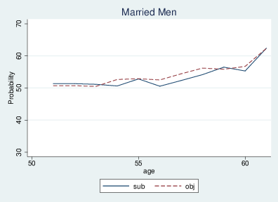
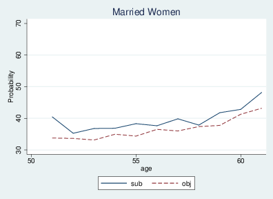
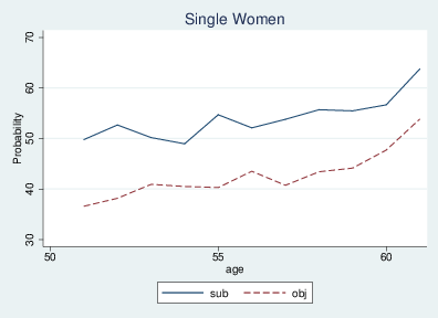
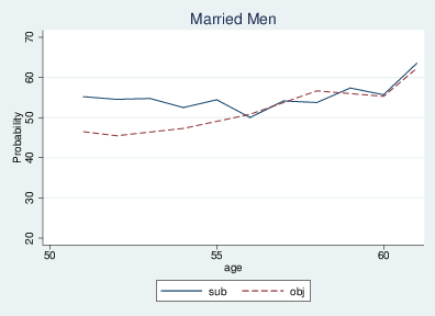
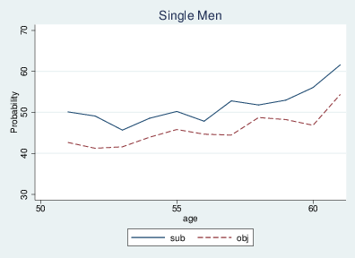
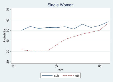
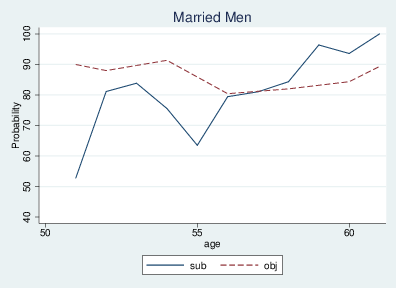
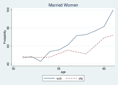
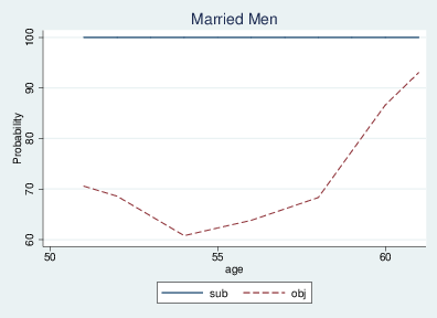
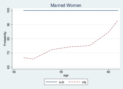
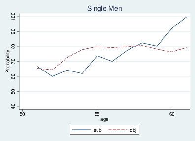
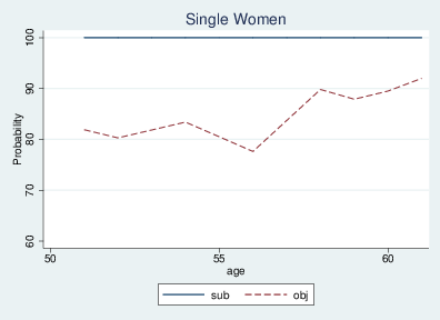
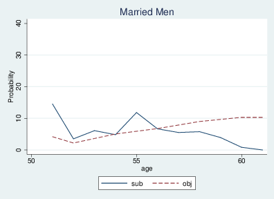
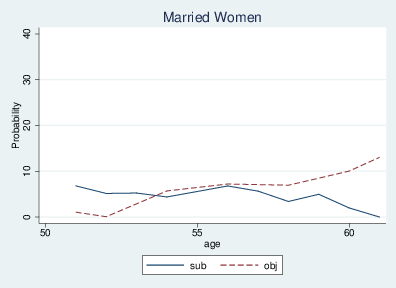
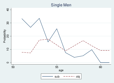
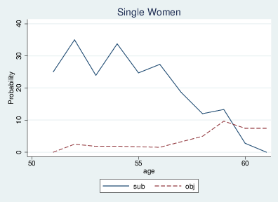
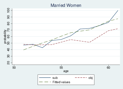
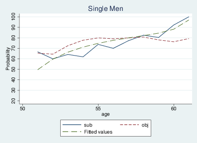
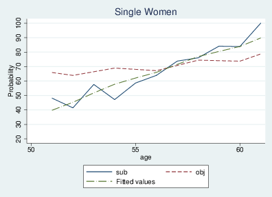
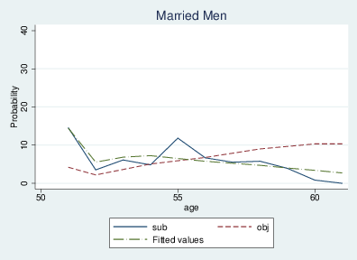
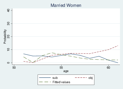
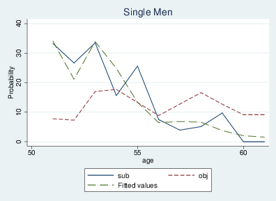
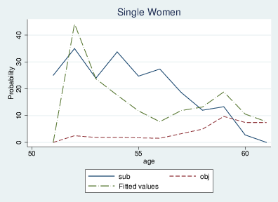
Figure 1 (in the Appendix) presents graphs with age on the x-axis and probabilities (objective and subjective) on the y-axis. With the exception of married men, whose subjective probabilities seem to correspond to the objective probabilities, all other groups tend to overestimate the probability of working full time after age 62. The effect seems most pronounced for single women. Subjective probabilities do not seem to converge to objective probabilities over time, with the average deviation remaining approximately constant between the ages of 51 and 61. This is in contrast to what would be predicted by the theory of Rational Bayesian Learning.
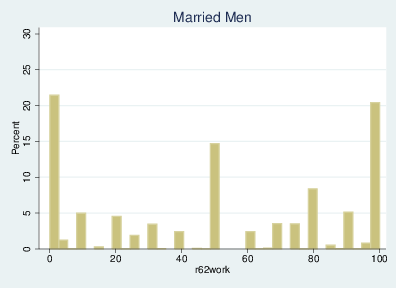
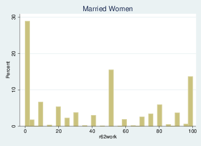
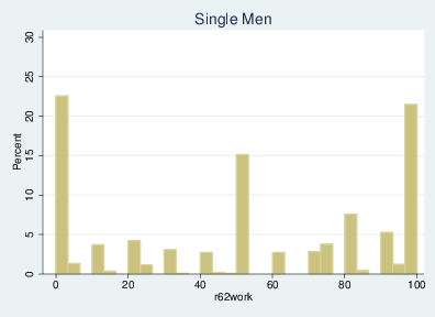
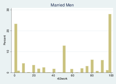
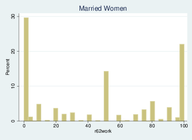
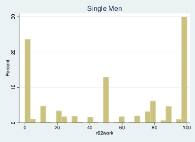
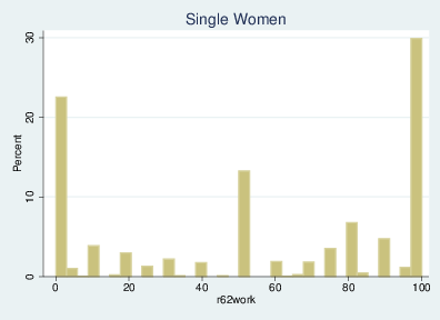
To try to ascertain the cause of this phenomenon, I examined the distribution of subjective probabilities at different ages for the different subgroups. Figures 2 and 3 display these distributions with the subjective probability given by respondents on the x-axis, and the frequency of each response given on the y-axis. There are two important observations. Firstly, there is a definite bunching of responses at 0, 50 and 100 percent for all four subgroups at both younger and older ages. Secondly, while the proportion of responses at 0 and 50 remains approximately constant at both younger and older ages, the proportion of responses at 100 increases for all our four groups as individuals get closer to age 62. This leads to the question: Are these increasing number of responses at 100 responsible for the lack of convergence of the subjective probabilities to the objective probabilities as individuals approach age 62?
In order to answer this question, all observations with extreme focal point responses (0 and 100) are omitted. Only focal values of 0 and 100 are omitted, not 50, since there is enough evidence in the empirical literature to suggest that answers of 0 and 100, specifically, demonstrate greater uncertainty than the rest of the sample. The interest of this paper is specifically in answers of 0 and 100.
The same methodology outlined in Section 3.3 is then carried out for this sample. Average subjective probabilities as well as objective probabilities are recalculated for this group.
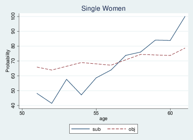
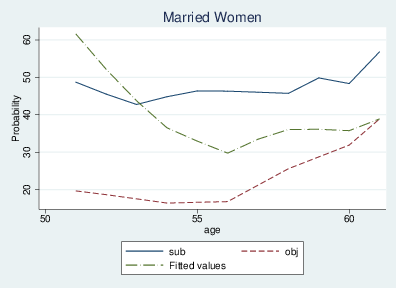
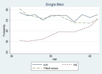
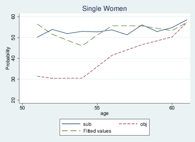
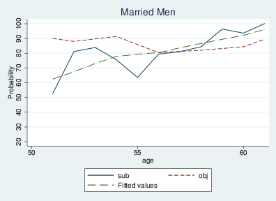
Figure 4 shows the relevant subjective and objective probabilities for this sample, with age on the x-axis and the relevant probabilities on the y-axis. A different picture emerges. There is definitely evidence that this sample of individuals are rational Bayesian learners. This is especially the case with single men, single women and married men, where by age 61 the subjective probability almost completely coincides with the objective probability. In the case of married women, some convergence is present, but it is not complete. This convergence is the case, despite the fact that such individuals start off far less accurate than the those in the sample including focal point respondents. What is important in the rational Bayesian learning paradigm is not the size of the initial bias but rather the fact that the bias decreases over time.
As a whole, it seems that individuals giving nonfocal answers (including answers at 50) tend to subscribe to the rational Bayesian learning paradigm, while the population as a whole (including those giving focal point answers of 0 and 100) does not.2 It is also apparent that, although the absence of focal point responses results in greater accuracy at ages closer to age 62, at younger ages the reverse effect is seen (the upward bias is smaller at younger ages in the entire sample than in this selected sample). In Section 4.2, the nature of focal point responses is analyzed more closely, showing how it is only certain types of focal point responses that are problematic. The larger bias at younger ages in the sample without focal points is due to leaving out the non-problematic (accurate) focal points.
This section looks at individuals whose last response to the question regarding the probability of working past age 62 was a focal point of either zero or 100. This last response could have been given either at age 61 (since this is the last time the question is asked), or the last time they answered the question before stopping to work. Either way, it is here, according to the rational Bayesian learning paradigm, that responses should be most accurate. It is incorrect responses that are of most interest here. I consider two types of individuals: those whose focal point response was updated from a nonfocal response given at a younger age, and those who gave the particular focal point response consistently over the time they were questioned.3
Table 1 shows the percentage of those “end point” focal point responses that were updated from nonfocal responses. We notice that, with the exception of married men, the proportion of zeros that arise from nonfocal responses is small relative to the proportion of 100’s that arise from nonfocal answers. We also notice that for married individuals a greater overall percentage of end-point focal responses arise from nonfocal answers.
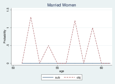
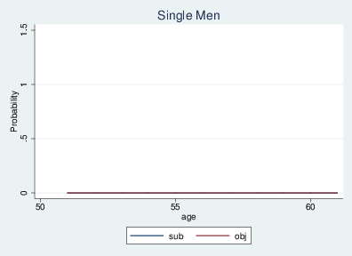
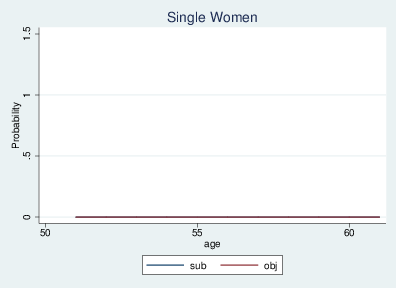
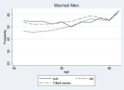
Figure 5 shows the sample of individuals whose focal point responses of 100 were updated from nonfocal answers. A definite increasing upward bias as age 62 approaches can be seen. The objective probabilities of working past age 62 for 61 year olds giving focal point responses of 100, are 78, 72, 79 and 89 percent for single women, married women, single men, and married men respectively. That means that only 78% of single women, 72% of married women, 79% of single men and 89% of married men who gave a focal point response of 100 that was updated from a nonfocal response actually worked past age 62. Figure 6 shows individuals giving a focal point response of 100 consistently over the time they were questioned. We see that as age 62 approaches, the focal point answer of 100 now becomes relatively accurate. In particular, over 90% of all individuals that gave a consistent focal point response of 100 since age 51, and were still working at age 61, actually worked past age 62.
Figure 7 shows individuals who give focal point responses of zero that arise from nonfocal responses. Here an increasing downward bias as age 62 approaches is noticed. The corresponding objective probabilities at age 61 are 8, 13, 9 and 11 percent for single women, married women, single men and married men respectively. In other words 8% of single women, 13% of married women, 9% of single men and 11% of married men that at age 61 thought there was zero chance of working past age 62 (even though at earlier ages they might have thought differently) did indeed work past age 62. The downward bias at age 61 is far smaller than the upward bias at the same age for focal point responses of 100 that arise from nonfocal responses.
Figure 8 shows individuals who give a focal point response of zero consistently over the time they were questioned. These individuals are remarkably accurate from the outset. Even at younger ages, the objective probability is equal to, or very close to zero. Virtually everybody who consistently felt that they would not work past age 62, was correct.
It is clear that it is focal point responses that arise from nonfocal responses that induce a bias at ages closer to 62. However, with the exception of married men, since the proportion of zeros that arise from nonfocal responses is small relative to the proportion of 100’s that arise from nonfocal answers (Table 1), as well as the fact that the upward bias is greater than the downward bias, it is an upward bias that is observed as age 62 approaches. In the case of married men, it is the fact that these proportions are essentially equal, and that the magnitude of the bias is essentially the same, that the upward and downward biases cancel, and that they thus appear “rational” at this point.
In the next section, a theoretical framework is provided that can explain the mechanism whereby bias is created as nonfocal responses become focal points.
It is assumed here that subjective probabilities are non-additive beliefs. Non-additive beliefs account for individuals exhibiting ambiguity attitudes in the sense of Schmeidler (1989). In particular, the non-additive belief is assumed to take the form of a neo-additive capacity in the sense of Chateauneuf et al. (2007).
A neo-additive capacity, v, represents a belief that has two components, a rational component and a psychological component. The rational component is the additive part of the capacity, and the psychological component puts some weighting on the belief that the event in question will occur with certainty. In the context of this paper, the capacity is given by
| v(E62)=100· (δ · λ )+(1−δ )· µ (E62) (1) |
where E62 is the event that the agent works past age 62, µ (E62) is the additive part of the capacity, δ є [0,1] (degree of ambiguity) measures the lack of confidence the decision maker has in the additive part of the capacity, and λ є 0,1] measures the weight the decision maker gives to the belief that he will, with certainty, work past age 62. (This belief is given by 100—indicating 100 percent chance.)
Now, for a given level of ambiguity, δ, the greater is λ , the more weight will be given to the belief that there is 100% chance of working past age 62. If λ=0, no weight is given to the belief that there is a 100% chance of working past age 62. If λ =1, a weight of δ will be placed on the belief that the agent will, with absolute certainty, work past age 62. If λ = 0, a weight of δ will be placed on the belief that an agent will with absolute certainty, not work past age 62. In both instances, a weight (1−δ ) will be placed on the additive probability, µ (E62), as it is perceived by the agent.
At the same time, as the level of ambiguity, δ , increases for a given level of λ , less weight is placed on the additive probability, µ (E62). If δ =0, the capacity reduces to the additive probability, and the agent is “rational”. If λ =1, the neo-additive capacity displays an upward bias from the additive probability, while if λ =0, it displays a downward bias. A neo-additive capacity with λ =1 is referred to here as an overestimating capacity, and a neo-additive capacity with λ =0, as an underestimating capacity. Intuitively, this tendency to overestimate or underestimate the probability of an event results from a psychological bias. It is a cognitive process that leads an individual to deviate from the objective evidence (which would lead to an objective/additive probability, µ (E62)), and form a belief that is influenced by this psychological bias.
At the same time it is assumed that there is a rational “bias” contained in the additive part of the capacity which decreases over time in line with the Rational Bayesian Learning paradigm. The bias is rational in the sense that individuals are not expected to have enough information in earlier years to know the objective probability of working past age 62. However, while such individuals are not expected to know the true objective probability at the outset, as they approach age 62 and gain more knowledge and experience, their assesment of the objective probability should converge to the true objective probability. In particular
| µ (E62)=φ62−j· π j,62 (2) |
where π j,62 is the objective probability that an agent of age j will work full time after age 62, and φ is a measure of the rational bias, where φ <1 implies that there is a rational underestimation, and φ >1 implies that there is a rational overestimation. As j→ 62, φ 62−j—→ 1 so that µ (E62)→ π j,62. That is, as the individual approaches age 62, the rational bias decreases so that the additive part of his capacity tends to the true objective probability.
In contrast, the psychological bias is seen to increase over time. Gilboa and Schmeidler (1993) and Eichberger et al. (2006) present various update rules for non-additive measures. The overestimating update rule results in a situation where λ jumps to 1 after one round of updating, and over time δ → 1 so that the capacity tends to 100. Indeed, a focal point answer of 100 can be interpreted as a neo-additive capacity in the extreme case where λ =1 and δ =1. Thus, individuals in the sample who update their non-additive belief according to the overestimating update rule will be inclined to give a focal point answer of 100 as time goes on.4 (Appendix B, Overestimating Update Rule, gives a more mathematically detailed description of how this process works.) The underestimating update rule results in a situation where λ jumps to zero after one round of updating, and over time δ → 1 so that the capacity tends to zero. Indeed, a focal point answer of zero can be interpreted as a neo-additive capacity in the extreme case where λ =0, and δ =1. Thus, individuals in the sample who update their non-additive belief according to the underestimating update rule will be inclined to give a focal point answer of zero as time goes on. (Appendix B, Underestimating Update Rule, gives a more mathematically detailed description.)
What might one say of the sample of individuals whose subjective measures converge to the corresponding objective measures over time (or as in the case of those giving a zero response consistently, coincide from the start)? While such beliefs are theoretically consistent with non-additive measures that are updated according to the Sarin-Wakker update rule (Sarin & Wakker, 1998), the implication that, for a neo-additive capacity, all ambiguity is eliminated after one round of updating, leads to preference for the more realistic interpretation that such measures are additive from the start. At the very least it can be assumed that, at the beginning of questioning, these beliefs are additive and are updated according to the rational Bayesian learning paradigm.
The population as a whole is comprised of these different groups of individuals, who update their subjective probabilities (capacities) according to these different update rules.5 As a whole, the population tends to behave like the representative agent discussed in Ludwig and Zimper (2013). This agent displays rational Bayesian learning, together with increasing psychological bias as time goes on. Since, as Table 1 shows, with the exception of married men, the number of individuals updating their responses according to the overestimating update rule is large compared to those updating according to the underestimating update rule, as well as the fact that the magnitude of the upward bias is greater than that of the downward bias, it is an increasing upward psychological bias that is observed in the population as a whole.
Parameters for the models proposed above were estimated using non-linear regression analysis. Non-linear regression analysis predicts observed data as a non-linear function of parameters of a model. The parameters are estimated based on the average subjective probabilities in each age group—that is, the aim is to fit the curves in the various diagrams above. Parameters were estimated for three different samples.
First, the φ parameter for a rational Bayesian learning model for the sample of individuals giving only nonfocal point responses was estimated. φ is a measure of the rational bias, with φ <1 implying there is a rational underestimation, and φ >1 implying there is a rational overestimation. Then, a model of “rational Bayesian learning, with psychological bias” consistent with updating according to the Overestimating update rule, for individuals who give focal point responses of 100 that have been updated from nonfocal responses, was estimated. Here φ , λ and δ were estimated. Again φ is a measure of the rational bias, λ є 0,1] is the weight given to the belief that there is a 100% chance of working past age 62, and δ є 0,1] is the initial level of ambiguity before updating. Lastly, a model of “rational Bayesian learning, with psychological bias” consistent with updating according to the Underestimating update rule, for individuals who give focal point responses of 0 that have been updated from nonfocal responses was estimated. Again φ , λ and δ are estimated, with the same interpretations as before.
In particular, the dependent variable is the subjective probability which is modelled as an additive belief corresponding to equation 2 for the sample giving only nonfocal point responses. The subjective probability is modelled as a neo-additive capacity, corresponding to equations 1, 3, 4 and 5 for the sample giving focal point responses of 100 updated from precise responses, and to equations 1, 6, 7 and 8 for the sample giving focal point responses of zero updated from nonfocal responses. For all tables, t values are in parentheses.
Table 2 presents estimates of φ (rational bias) for the sample of Bayesian learners, while Figure 9 shows the actual and predicted values of the subjective probabilities The predicted values are based on the estimates of φ given in Table 2. In all instances there is an initial overestimation (φ >1), with the fit of the model being very good. Note the high R2 values, as well as the fitted curves in Figure 9. Table 3 presents the estimates for the sample of individuals who give focal point responses of 100 that have been updated from nonfocal responses. There is an initial underestimation in all cases ( φ <1). The R2 values, as well as the fitted curves (based on our estimates of λ , δ and φ ) in Figure 10 show a very good fit. In Table 4 the estimates of φ λ and δ for the sample of individuals who give focal point responses of zero that are updated from nonfocal answers. There is an initial overestimation. The R2 values and Figure 11 show that the fit is better for men than for women.
Noticeable is that despite the fact that the sample in Table 4 end up with answers of zero, while the sample in Table 3 end up with responses of 100, their initial values of λ are not hugely different. Thus, despite the fact that their initial attitudes towards ambiguity are not so different, it is the way that they interpret new information that determines what kind of answer they give closer to age 62.
The aim of this paper is to show that the formal interpretation of focal point answers as non-additive measures—and in particular as neo-additive capacities—is consistent with the features of the data. In fact, the fit of the data to the models is very good.
Focal point responses of 100 or 0 closer to age 62 that are updated from nonfocal responses are biased upwards and downwards respectively. A focal point response of 100 or 0 that is updated from a nonfocal response can be represented by a neo-additive capacity. A neo-additive capacity is a non-additive belief that represents a deviation from an additive belief, such that the degree of ambiguity measures the lack of confidence the agent has in some additive probability distribution. As this belief is updated over time according to either the Underestimating or Overestimating Update Rules, the degree of ambiguity increases, in that the agent has decreasing confidence in the additive probability distribution. In the context of this paper, the agent then resolves this ambiguity by having complete confidence in the extreme belief that he/she will, as in the case of the Overestimating Update Rule or will not, as in the case of the Underestimating Update Rule, with absolute certainty, continue to work full time after age 62.
Individuals who consistently give nonfocal responses, or who consistently give focal point responses over the time they are questioned, are rational, in the sense that their subjective probabilities coincide with the objective probabilities, at least by the time they are close to age 62. While, theoretically, these beliefs are consistent with non-additive measures updated according to the Sarin-Wakker Update Rule, they are also consistent with additive probabilities. Given the fact that Sarin-Wakker updating implies that all ambiguity disappears after one round of updating, it is probably more appropriate to represent these beliefs as additive measures.
This result, together with the observation that, with the exception of married men, the proportion of zeros that are updated from nonfocal responses is small relative to the proportion of 100’s that are updated from nonfocal answers, as well as the fact that the magnitude of the upward bias is greater than that of the downward bias, explains the persistence of the upward bias in the sample of the population as a whole, even as age 62 approaches.
It should be noted that, while it appeared at the outset that married men were more rational than other individuals in the sense that their subjective probabilities seemed to converge completely to their objective probabilities by age 62, after decomposing the data further, this can be seen not to be the case. The absence of an upward bias in the subjective probability of working past age 62 close to age 62 for married men is not due to their being more rational, but rather to the positive and negative biases of focal points of 100 and 0 respectively cancelling each other out, as illustrated in Table 1.
Finally, while this paper shows that individuals update their beliefs differently, future research will aim at identifying the reasons for such differences in the updating process.
Basset, W. F. & Lumsdaine, R. L. (2001). Probability limits Journal of Human Resources, 36(2), 327–363.
Bloom, D., Canning, D., Moore, M., & Song, Y. (2007). The effect of subjective survival probabilities on retirement and wealth in the US. In Robert Clark, Andrew Mason and Naohiro Ogawa (eds), Population aging, intergenerational transfers and the macroeconomy.
Börsch-Supan, A. (1998). Subjective survival curves and life cycle behavior. In D. A Wise (Ed), Inquiries in the economics of aging, 306–309, Chicago University Press.
Bruine de Bruin, W., Fischhoff, B., Millstein, S. G., & Halpern-Felsher, B. C. (2000). Verbal and numerical expressions of probability: Its a fifty-fifty chance. Organizational Behavior and Human Decision Processes, 81, 115–131.
Chateauneuf, A., Eichberger, J., & Grant, S. (2007). Choice under uncertainty with the best and worst in mind: Neo-additive capacities. Journal of Economic Theory, 127, 538–567.
Eichberger, J., Grant, S., & Kelsey, D. (2006). Updating Choquet beliefs. Journal of Mathematical Economics, 43, 888–899.
Gilboa, I., & Schmeidler, D. (1993). Updating ambiguous beliefs. Journal of Economic Theory, 59, 33–49
Hill, D., Perry, M., & Willis, R. (2004). Estimating Knightian uncertainty from survival probability questions in the HRS. Unpublished Manuscript, University of Michigan.
Hurd, M. D., & McGarry, K. (1993). Evaluation of subjective probability distributions in the HRS. Working Paper 4560, National Bureau of Economic Research, Cambridge, MA.
Hurd, M. D., & McGarry, K. (1995). Evaluation of the subjective probabilities of survival. Journal of Human Resources, 30 (supplement), 268–292.
Hurd, M. D., McFadden, D., & Gan, L. (1998). Subjective survival curves and life cycle behavior. In David Wise (ed), Inquiries in the economics of aging, Chicago: University of Chicago Press.
Hurd, M. D. (2009). Subjective probabilities in household surveys. Annual Review of Economics, Annual Reviews, 1(1), 543–564.
Hurd, M. D., Reti, M. & Rohwedder, S. (2009). The effect of large capital gains or losses on retirement. In David Wise (ed), Developments in the economics of aging, NBER Chapters.
Huynh, K. P., & Jung, J. (2010). Correcting focal point biases in subjective health expectations. Mimeo, Towson University.
Kleinjans, K. J., & Van Soest, A. (2010). Nonresponse and focal point answers to subjective probability questions. IZA Discussion Papers 5272, Institute for the Study of Labor (IZA).
Lillard, L. A., & Willis, R. J. (2001). Cognition and wealth: The importance of probabilistic thinking. Michigan Retirement Research Centre, Research paper no, WP 2001-007.
Ludwig, A., & Zimper, A. (2013). A parsimonious model of subjective life expectancy. Theory and Decision, 75(4), 519–541.
Ludwig, A., & Zimper, A. (2009). On attitude polarization under Bayesian learning with non-additive beliefs. Journal of Risk and Uncertainty, 39(2), 181–212.
Manski, C. F., & Molinari, F. (2010). Rounding probabilistic expectations in surveys. Journal of Business and Economic Statistics, 28(2), 219–231.
Romm, A. (2014). The effect of retirement date expectations on pre-retirement wealth accumulation: The role of gender and bargainning power in married US households. Forthcomming, Journal of Family and Economic Issues.
Sarin, R., & Wakker, P. P. (1998). Revealed likelihood and Knightian uncertainty. Journal of Risk and Uncertainty, 16(3) , 223–250.
Schmeidler, D. (1989). Subjective probability and expected utility without additivity. Econometrica, 57, 571–587.
Willis, R. (2005). Discussion of Li Gan, Michael Hurd and Daniel McFadden, Individual subjective survival curves. In David Wise, Ed. Analysis in the economics of aging. University of Chicago Press.
The objective probabilities are calculated by observing the cohorts over time. In particular, the objective probability of working full time after age 62 for a cohort of individuals who are, say, 52 and working in 1992, is based on what this cohort of individuals was doing in 2002 when they were 62. Thus, for this cohort, only individuals who are still in the sample in 2002 are included. Similarly, the objective probability for a cohort of individuals aged 52 in 2002 is based on what they are expected to be doing in 2012 when they are 62. The objective probability for a cohort of 52 year old single working males in 1992, say, is calculated by looking at the proportion of this group that is working full time in 2002 when they are age 62. For a cohort of 54 year olds in 1992, the proportion working full time in 2000 is considered.
This is easily done for ages that are even numbers, not so easily done for ages that are odd numbers. For example, 53 year old individuals in 1992 were 62 in the year 2001. However, there was no HRS survey in 2001, so we cannot ascertain what this cohort was doing at age 62. Thus, the objective probabilities for odd ages are interpolated (linearly) from the even ages.6
In order to calculate the objective probabilities for 62 year olds after 2004, the predicted trends in labor force participation rates at age 62, calculated by the Bureau of Labour Statistics (BLS), are used in order to predict the HRS proportions up till 2016. Since the trend in the proportion of 62 year olds working full time in the HRS data has greatly followed the trends calculated by the BLS for the population as a whole, it can be assumed that, at the time the HRS was carried out, a rational agent would expect that barring any shocks, the trends in the HRS proportions would follow the trends predicted by the BLS. Thus, existing HRS proportions up until 2004 are used, and then from these, proportions up till 2016 are extrapolated, using BLS trends.
We extrapolate using these BLS trends for two reasons. Firstly, we cannot calculate objective probabilities directly from the HRS for years for which we dont have HRS data. Secondly, the financial crisis of 2007–2008 was a massive structural break causing significant changes in objective retirement probabilities. Our respondents in 2004 and before could not have realized this would occur, and a rational assesment of the objective probability of working past age 62, at the time they were questioned, would have been based on what would have been expected given historical and forecasted trends.
A complication arises from an ambiguity in the question, “What is the probability that you will be working full time after age 62?” Does this imply after the individual’s 62nd birthday, or does it imply after the individual is no longer 62? The method used to calculate the objective probability discussed above assumes the first interpretation. However, as noted by Hurd and McGarry (1993), some individuals assume the first interpretation, others the second. Thus, I also calculated the objective probability under the second interpretation. I calculated the proportion of a certain cohort working at time t that was working full time at age 63. Here of course there is information on the odd ages, and interpolation needs to be carried out for the even ages.
The final objective probability for each cohort used in the analysis is the average of those calculated under the first and second interpretations.
Application of The Overestimating Update Rule to estimator (1), results that after gathering h years more experience and information (denoted Ih),
| v(· |Ih)=100· δ Ih+(1−δ Ih)· µ (· |Ih) (3) |
such that
| δ Ih= |
| (4) |
for λ ∈ (0,1], and
| µ (· |Ih)= | ⎛ ⎜ ⎜ ⎝ |
| ⎞ ⎟ ⎟ ⎠ | · πj,62 (5) |
where v(· |Ih) represents the agent’s posterior belief that he will work full time after age 62 given the information he has after h years experience (Ih), δ Ih represents the level of ambiguity after the h years experience, and is related to the initial level of ambiguity, δ , by Equation 4, and µ (Ih) is the agent’s perception of the additive probability after h years experience. It is assumed here for simplicity that the agent starts learning at age 51, such that age 51 corresponds to h=1. Proof of equation 4 is derived by Ludwig and Zimper (2009, p. 205, proof of observation 4, “optimistic update rule”). Finally equation 5 is analogous to equation 2, just taking h into account. This is proved in Ludwig and Zimper (2013, assumptions 1 to 4 and proposition 2). As j→ 62, µ (· |Ih)→ π j,62 (i.e. the agent’s perception of the additive (objective) probability tends to the true objective probability.).
It can be seen that λ Ih=1. Thus, regardless of the initial value of λ , after updating, λ jumps to 1 so that the individual’s capacity reflects overestimation. At the same time, following Ludwig and Zimper (2013, assumptions 1 to 4 and proposition 2), it can be shown that µ (Ih)=( 1/1+h) . Essentially this results from the fact that agents are gaining experience through a series of Bernoulli trials, where they observe the proportion of individuals working past age 62 in each trial (year). Ludwig and Zimper show that the expected probability tends to ( 1/1+h) .
Since µ (Ih) gets smaller as h increases, δ Ih>δ Ih−1. Thus, as time goes on, and the agent gathers more and more information, δ → 1, so that his capacity tends to 100. Indeed, a focal point answer of 100 can be interpreted as a neo-additive capacity in the extreme case where λ =1, and δ =1. Thus, individuals in the sample who update their non-additive belief according to the overestimating update rule will be inclined to give a focal point answer of 100 as time goes on.7
Application of the Underestimating Update rule to belief (1) results that
| v(· |Ih)=(1−δ Ih)· µ (· |Ih) (6) |
such that
| δ Ih= |
| (7) |
for λ ∈ 0,1), and as before
| µ (· |Ih)= | ⎛ ⎜ ⎜ ⎝ |
| ⎞ ⎟ ⎟ ⎠ | · πj,62 (8) |
The proof of equations 6 and 7 can be seen in Ludwig and Zimper (2009, p. 205, proof of observation 5, “pessimistic update rule”). Thus, for any initial value of λ , λ Ih=0, i.e., after updating according to the underestimating update rule, λ jumps to zero. Also, δ h>δ h−1 i.e., the level of ambiguity increases after updating. Thus, as time goes on, and the agent gathers more and more information, δ → 1. Indeed, a focal point answer of 0 can be interpreted as a neo-additive capacity with λ =0, and δ =1. Thus individuals in the sample who update their non-additive belief according to the underestimating update rule will be inclined to give focal point answer of 0 as time goes on.
Copyright: © 2014. The authors license this article under the terms of the Creative Commons Attribution 3.0 License.
This document was translated from LATEX by HEVEA.