Birnbaum (2011) criticized tests of transitivity that are based entirely on
binary choice proportions. When assumptions of independence and stationarity
(iid) of choice responses are violated, choice proportions could lead to wrong
conclusions. Birnbaum (2012a) proposed two statistics (correlation and variance
of preference reversals) to test iid, using random permutations to simulate
p-values. Cha, Choi, Guo, Regenwetter, and Zwilling (2013) defended
methods based on marginal proportions but conceded that such methods wrongly
diagnose hypothetical examples of Birnbaum (2012a). However, they also
claimed that “true and error” models also satisfy independence and also fail
in such cases unless they become untestable. This article presents correct
true-and-error models; it shows how these models violate iid, how they might
correctly identify cases that would be misdiagnosed by marginal proportions,
and how they can be tested and rejected. This note also refutes other
arguments of Cha et al. (2013), including contentions that other tests failed
to violate iid “with flying colors”, that violations of iid “do not
replicate”, that type I errors are not appropriately estimated by the
permutation method, and that independence assumptions are not critical to
interpretation of marginal choice proportions.
Keywords:
1 Introduction
Although there is much to admire in the approach of Regenwetter, Dana, and
Davis-Stober (2011) for testing transitivity in choice experiments, Birnbaum
(2011) criticized its focus on marginal choice proportions rather than response
patterns. Birnbaum pointed out that when choice responses are not independent
and identically distributed (iid), any method based strictly on marginal choice
proportions could easily reach wrong substantive conclusions.
The main problem is that data generated from mixtures that include intransitive
preference patterns can appear to satisfy transitivity by such methods.
Birnbaum (2011) therefore suggested that one should analyze response patterns
or at least, that iid should be tested before drawing any conclusions about
transitivity from marginal choice proportions. Regenwetter, Dana,
Davis-Stober, and Guo (2011) replied that, when response patterns are to be
analyzed, one must collect more extensive data, and they stated that they were
unaware of statistical tests of iid for small samples, such as the little study
by Tversky (1969), or the small replication by Regenwetter et al. (2011).
Birnbaum (2012a) proposed two statistics using Monte Carlo simulation
methods (based on Smith and Batchelder, 2008) to test iid with small
samples. One statistic is the correlation coefficient between
preference reversals and the gap in time between two presentations of
the same choice problems. The other is the variance of preference
reversals between responses to the same problems in different blocks
of trials. These two statistics were designed to detect violations of
iid that would occur if people systematically changed their true
preferences during the study. Reanalysis via these two tests
indicated that the data of Regenwetter et al. (2011) violate the
assumptions of iid. Violations of iid might arise from many different
sources, including the possibility that a true-and-error (TE) model
describes responses in choice tasks.
Cha, Choi, Guo, Regenwetter, and Zwilling (2013) defended methods
analyzing only marginal proportions but they conceded that those
methods wrongly diagnose hypothetical examples presented by Birnbaum
(2012a). However, they falsely claimed that TE models also assume iid
and would therefore also fail to correctly diagnose such cases. They
next claimed if a TE model allowed a person to change “true”
preferences between blocks (to violate iid), the model would become
untestable and therefore useless. These statements and others in that
paper need to be corrected, because TE models violate iid,
they correctly diagnose such hypothetical examples, and yet they are
testable.
2 True-and-error models
Cha et al. (2013, p. 67) claimed
that the “standard true-and-error model” satisfies independence. However, I
specifically argued that violations of iid are produced in TE models within an
individual’s data when the same person changes “true” preferences from block
to block (Birnbaum, 2011, p. 680) and that iid could also be violated
between-persons when different people have different “true” preferences
(Birnbaum, 2011, p. 679). The so-called “standard” true-and-error model
presented by Cha et al. is merely a special case of the TE model in which
there is only a single true preference pattern and not a mixture.
A brief history of these models might be useful.
The models now called “true and error” trace their development to a paper by
Lichtenstein and Slovic (1971), who wished to state a clear null hypothesis in
which preference reversals between two ways of evaluating lotteries could be
analyzed. Sarah Lichtenstein developed the basic concepts from “common
sense” (Slovic, 2013 and Lichtenstein, 2013, April 3, personal
communications).
A paper by Conlisk (1989, Appendix I) presented a very clear statement of a
simpler form of their model, which was used to justify the statistical test of
correlated proportions, which has been the standard test whether or not choice
proportions in two choice problems are significantly different. In his version
of the model, it was assumed that all choice problems had the same rate of
error (whereas the earlier model of Lichtenstein & Slovic [1971] allowed that
choice and bidding tasks might have different rates of error).
Harless and Camerer (1994) applied the assumption of a single error
rate and stated that a more elaborate theory had not yet been
developed. The theory of homogeneous error rates has sometimes been
called the “tremble” theory because it seemed to say that response
errors arise between intention and response, as if the only reason for
pushing the wrong response key was the result of a “trembling hand”.
However, that interpretation is not necessary and might be misleading,
because errors more likely arise earlier in processing (Birnbaum,
2011). A person might misread the problem, misremember the
information, misaggregate the information, misremember the decision,
or push the wrong key, any of which could produce an error. Some of
the rival models of error have been reviewed and analyzed by Wilcox
(2008), Carbone and Hey (2000), and Loomes and Sugden (1998).
When testing transitivity, the constant-error-rate version implies
that inequality of different types of intransitive preference patterns
could be taken as evidence for a violation of transitivity
(Loomes, Starmer, & Sugden, 1991). Sopher and Gigliotti (1993)
disputed this interpretation, however, noting that, if error rates for
different choice problems are not equal, then asymmetry of different
types of cycles would not qualify as evidence of systematic
intransitivity. Their approach could, in turn, be criticized because
the model had (in principle) more parameters than degrees of freedom
in the data to which it would be applied. Perhaps this limitation is
why someone might claim that these models become untestable.
However, as noted in several recent papers (Birnbaum, 2011, p. 678; Birnbaum &
Bahra, 2012a; Birnbaum & Schmidt, 2008; Birnbaum & LaCroix, 2008), the use of
replications, as proposed by Birnbaum (2004) and improved upon in subsequent
papers, provides a way to estimate error rates that may differ for different
choice problems and still leave degrees of freedom to test the model. In
particular, it is assumed that repetitions of the same choice problem by the
same person in the same block of trials are governed by the same true
preferences and differ only because of error.
In tandem with these theoretical developments, recent empirical
results forced consideration of models that can violate iid (in
contrast to earlier models, which did not allow violation of iid).
Birnbaum and Bahra (2007b) reported cases where individuals perfectly
reversed preferences on twenty out of twenty choice problems between
blocks of trials; such cases are extremely unlikely given the
assumption of iid within a person. Instead, it seems more plausible
that individuals changed true preferences from block to block.
Birnbaum and Bahra (2012b) repeated the experiment with different
people and varied procedures and continued to find perfect reversals
and other strong evidence against iid. Birnbaum (2011, 2012a) noted
that, if a person changed “true” preferences during a long study, it
could create violations of iid. When iid is violated, marginal choice
proportions might be misleading.
That is the crux of Birnbaum’s (2011) criticism of the approach of
Regenwetter et al. (2011), which was focused on binary choice
proportions. Cha et al. (2013) did not accurately describe
appropriate TE models. I describe here how one can apply TE models to
the investigation of transitivity, if one is willing to do a more
up-to-date study than that done by Tversky (1969). I will describe
how such a study can be used to test iid, the TE models, and
transitivity.
I dispute other assertions by Cha et al. (2013) concerning
algorithms for testing iid via Monte Carlo simulation in Appendix A;
but first, let us consider the simplest TE model for the simplest case
to show that it violates response independence, even though the errors
are independent.
2.1 One choice problem presented twice per block
Imagine that one person is asked to respond to many different choice problems,
and embedded in each block of, say, 50 trials (which include many different
choice problems), a given choice problem (between A and B) is
presented twice, separated by many other intervening choice problems that are
termed fillers within each block. Each block is separated by another
task that requires, for example, 50 trials of other choice problems, called
separators. This study might be done with a different block of trials
on each of several different days.
The two versions of the same choice problem are denoted Choices AB and
A′B′. They might differ only in which button should be pressed in
order to respond that A is preferred to B. The use of
repetitions within blocks adds constraints that make TE models highly testable.
This experimental paradigm is similar to that used by Birnbaum and Bahra
(2012b, Exp. 3). [The design of Tversky (1969) and the replication by
Regenwetter et al. (2011) did not include repetitions within blocks.]
Table 1: A hypothetical table of results to responses by the same person to the
same choice problem presented twice each in 20 blocks of trials.
Blocks
Choice AB
Choice A′B′
1
0
0
2
0
0
3
0
0
4
0
0
5
0
0
6
0
0
7
0
0
8
0
0
9
1
1
10
1
1
11
1
1
12
1
1
13
1
1
14
1
1
15
1
1
16
1
1
17
1
1
18
1
1
19
1
1
20
1
1
Marginal choice proportion
0.6
0.6
Table 1 shows a hypothetical matrix of responses, where “0” indicates that the
person chose alternative A or A′ and “1” indicates a
preference for B or B′. Each row represents a different
block of trials, and the two entries within each row represent the responses to
the two, separated presentations of the same choice problem in the same block.
The marginal choice proportions are the column sums, divided by the number of
blocks (20). The two marginal choice proportions are each 0.6.
Let each response combination in a block (row of Table 1) be called a
response pattern. There are four possible response patterns:
00, 01, 10, and 11. In order to be
consistent within a block, the person had to push opposite buttons on separate
trials to indicate preference for A and A′ (00), or
for B and B′ (11).
Table 2: Data from Table 1 are organized in a cross-tabulation to evaluate
independence. These data violate independence, because products of marginal
proportions fail to reproduce joint proportions.
Response to Choice A′B′
Response to Choice AB
0
1
0
8
0
1
0
12
If response independence held, the probability of each response pattern
would be given by the product of the marginal probabilities. For these data,
the predicted proportion for 11 would be (.6)(.6) = .36, and the
predicted proportion of reversals 01 or 10 would be (.4)(.6)
+ (.6)(.4) = 0.48. However, Table 2 shows that the response patterns do not
satisfy independence. Instead, the proportion of 11 was 0.6 (instead
of 0.36), and this person was perfectly consistent within blocks (0%
reversals, instead of 48%), thereby violating response independence.
By either the Fisher exact test on Table 2, or by means of Birnbaum’s (2012a)
test on the variance of preference reversals between blocks (on Table 1), one
can reject response independence with p < .0001. In every
case where this person chose A in a block, that same person chose
A′ in the same block, and in every block where the person chose
B, that person chose B′. This person was perfectly
consistent within blocks but changed preferences between blocks, resulting in
violations of response independence.
A second, sequential type of violation of iid is also apparent in the Table 1.
In particular, this person chose A and A′ on every choice for
the first 8 blocks and then switched to choosing B and B′.
Something changed over trials, resulting in a systematic violation of
stationarity within each column. This type of sequential violation is detected
by Birnbaum’s (2012a) correlation test, which evaluates the correlation
coefficient between the mean number of preference reversals between rows and
the gap (in blocks) between rows. In this case, the correlation, r =
0.94, and p < .0001.
These two statistics show that the data in Table 1 systematically violate the
assumptions of independence and stationarity (a.k.a., iid), but they do not say
how or why. One model that can describe certain violations of independence
(but not all) is the true-and-error (TE) model.
2.2 True-and-error model for One Choice Problem Repeated in Each Block
A TE model can be expressed for this situation as follows: Suppose that two
responses by the same person to the same choice problem within a block are
governed by the same “true” preferences, except for random error, and suppose
that responses in different blocks might be governed by different “true”
preferences (Birnbaum, 2011; Birnbaum & Bahra, 2012a).
Suppose that if the person is in the “true state” of preferring A the
error probability is e, which is the probability of choosing
B when the true preference is A. Assume that if the person
is in the “true state” of preferring B, that the probability of
making an error is also e. Suppose that the probability of being in
the state of truly preferring B is p. Assume that p
and the error rate, e, are stationary (remain constant) throughout the
study, that errors are mutually independent, and that e <
½.1
Do these iid assumptions concerning p and e mean that choice
responses are independent, as in the so-called “standard true-and-error
model” by Cha et al. (2013)? No, absolutely not. This TE model violates
response independence, as shown next.
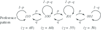
The predicted probabilities of the four response patterns are as follows:
P(00) = p(e)(e) +
(1–p)(1–e)(1–e) (1)
P(01) = P(10) = e(1–e) (2)
P(11) = p(1–e)(1–e) +
(1–p)(e)(e) (3)
P(11) is the predicted probability in the TE model for showing
the response pattern 11 in a block, p is the probability of
“truly” preferring B and B′, and e is the
probability of a random error. The marginal choice probability of choosing
B in a single AB choice problem is given as follows:
P(1*) = P(10) + P(11) =
p(1–e) + (1–p)e, where
P(1*) is the marginal, binary probability of choosing
B over A.
Do Equations 1–3 satisfy response independence? That is, can we write
P(11) = P(1*)P(*1)? No.
If p = .6 and e = 0, for example, this model is perfectly
consistent with the data of Table 2 that systematically violate response
independence.
This violation of response independence by the TE model does not require the
error rate to be zero; for example, if p = 0.63 and e = 0.11,
then P(1*) = P(*1) = 0.6, so
P(1*)P(*1) = 0.36, whereas
P(11) = 0.50.
So even though errors are independent of each other, responses are not predicted
to be independent, except in special cases, such as when p = 1. Put
another way: even though probability of the conjunction of two errors is
represented by the product of their probabilities, the probability of a
conjunction of two responses is not given by the product of response
probabilities, but instead by Equations 1–3.
Cha et al. (2013, Equation 6) presented a model that satisfies
response independence and called it the “standard true-and-error”
(STE) model. Independence can hold in special cases of TE, such as
when p = 1, but Expressions 1-3 do not satisfy independence
in general (Birnbaum, 2011). The Cha et al. STE model is not a
standard TE model; instead, it is only a special case in which there
is only one true preference pattern; that model is not relevant to
this debate, as noted by Birnbaum (2011, p. 680).
Cha et al. (2013, p. 70) next claimed that if a TE model allowed that people
changed true preference between blocks (to account for violations of iid), the
TE model would become un-testable. That claim is also false, even in this
simplest case of a single choice problem, as shown next.
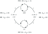
Table 3: Hypothetical cross-tabulations illustrating that response independence
and TE independence can be separately satisfied or violated by repeated
responses to a single choice problem. Both models are satisfied in the example
in the upper left and both are violated in the case in the lower right.
Independence satisfied
Independence violated
TE satisfied
A′
B′
A′
B′
A
16
24
30
10
B
24
36
10
50
TE violated
A′
B′
A′
B′
A
8
32
20
25
B
12
48
5
50
Table 3 displays four different hypothetical cross-tabulations of a repeated
choice to show that response independence and error independence can separately
fly or fail; that is, failure or satisfaction of one neither guarantees nor
refutes the other. (Entries in Table 3 sum to 100, so they can be viewed as
percentages, or divided by 100 to facilitate calculations on proportions).
Each of these models (independence and TE) can be tested by a Chi-Square on the
same 2 × 2 array with 1 df, since each model uses two parameters. Response
independence implies that each cell entry can be reconstructed from the row and
column marginal proportions, and TE says that each entry can be reconstructed
from p and e, using Equations 1-3.
Table 4: Hypothetical data in a test of transitivity for a single person who
receives three choice problems twice in each of 20 blocks of choice problems,
where each of the six choice trials was separated by many filler trials and
each block of trials was also separated by multiple separator trials.
Choice Problems
Blocks
AB
BC
CA
A′B′
B′C′
C′A′
1
0
0
0
0
0
0
2
0
0
0
0
0
0
3
0
0
0
0
0
0
4
0
0
0
0
0
0
5
0
0
0
0
0
0
6
0
0
0
0
0
0
7
0
0
0
0
0
0
8
0
0
0
0
0
0
9
1
1
1
1
1
1
10
1
1
1
1
1
1
11
1
1
1
1
1
1
12
1
1
1
1
1
1
13
1
1
1
1
1
1
14
1
1
1
1
1
1
15
1
1
1
1
1
1
16
1
1
1
1
1
1
17
1
1
1
1
1
1
18
1
1
1
1
1
1
19
1
1
1
1
1
1
20
1
1
1
1
1
1
Marginal choice proportion
0.6
0.6
0.6
0.6
0.6
0.6
In the two examples in Table 4 that perfectly satisfy response independence,
each entry can be perfectly reproduced as the products of their marginal choice
proportions.
In the two examples of Table 4 that violate response independence, people are
more consistent than expected (i.e., the entries on the major diagonal are
greater than expected from products of marginal proportions). In the two cases
violating TE, the matrices are not symmetric (i.e., one type of preference
reversal between replications is more probable than the other).
Treating the hypothetical entries in the tables as observed frequencies, the
χ2(1) for cases violating independence are 34.0 and
16.5 in the first and second rows, respectively. The
χ2(1) for examples violating TE are 9.66 and 22.14,
respectively. The critical value of χ2(1) with
α = .01 is 6.63, so each of these would be considered “significant”.
In the two cases satisfying TE, the parameters are p = 1 and
e = .4 in the case that also satisfies response independence and
p = .63 and e = 0.11 in the case that violates response
independence. Chi-Squares are zero for models that fit
perfectly.2
These four examples refute the claims by Cha et al. (2013) that the standard TE
model implies independence, and they refute the claim that if TE models
violated independence, they would be rendered un-testable. See also Birnbaum
and Bahra (2012a, pp. 407–408), including their example in which the TE model
would be rejected.
2.3 True-and-error model with multiple subjects and one block each
Now suppose that the data in Table 1 instead represented results from 20
different participants, each of whom participated in only one block
(instead of 20 blocks by the same person). That is, suppose each row of Table
1 represents responses by a different person, tested separately. What is the
“standard” TE model for that situation? In that case, Equations 1–3 are the
same, but the interpretations of parameters differ. It is again assumed that
the same person in the same block of trials is governed by the same “true”
preferences, but in this case, it is assumed that different people might have
different “true” preferences. In this case, p represents the
proportion of people who “truly preferred B” in their first (and
only) block. In this case, violation of independence arises because different
people have different “true” preferences.
To emphasize the distinction between these two cases, Birnbaum and Bahra (2012a)
used the terms iTET (individual True and Error Theory) and
gTET (group True and Error Theory) to denote cases where
violations of iid arise from an individual changing preferences from block to
block (iTET) and where violations of iid arise from individual
differences in a group of people (gTET), respectively. Both of these
cases were discussed in Birnbaum (2011, p. 679) and Birnbaum (2011, p. 680),
respectively.
In the simplest version of gTET, e represents an error
rate that is assumed to be the same for all persons. When there are different
people, however, one might hypothesize that different people might have
different amounts of noise in their data, so violations of this assumption
might show up as violations of this model. Indeed, Birnbaum and Gutierrez
(2007) found evidence that this simple model could be rejected in favor of a
more complex model in which different people had different error
multipliers.3
In iTET, stability of e means that the individual maintains
the same error rate throughout the study, which would be violated in cases
where a person becomes better with practice or where she might become fatigued
over trials. It is important to realize that these theorized violations of the
model can be tested against more general models that allow the violations of
these assumptions.
It is also important to keep in mind that violations of independence in
these two cases, as interpreted by the iTET and gTET models
come from different origins. So even though the equations are the same, the
violations of independence have different empirical interpretations.
For example, the correlation test proposed by Birnbaum (2011, 2012a) is really
anticipated to be violated only in the case of iTET, because that
statistic is sensitive to violations of iid that arise from sequential effects;
that is, preference reversals between rows that are related to the temporal
separation between blocks. If that test were to show significant violations in
the gTET paradigm, it would mean that the order in which people were
tested somehow affected the results, for example, that participants
communicated via some type of ESP that depended on the sequence in which they
were tested. Therefore, the data of Table 1 are not realistic for the
gTET situation, if the rows represented the order in which different
participants were separately tested. A more realistic example for
gTET could be created from Table 1 by randomly switching rows, which
would create a random sequence within each column; however, that resorting of
rows would preserve the same cross-tabulation as in Table 2.
At this point, it is also worthy of note that, whereas the results in Table
2 are perfectly consistent with iTET, that model does not allow one to
predict nor to fit the sequential information in the data of Table 1. In order
to describe the obvious sequential effects in Table 1, one would need
additional theory, such as that proposed by Birnbaum (2011, p. 680), and
described more fully here in Appendix B. For example, one might theorize that
the parameters of a decision making model (such as the TAX model of Birnbaum,
2008) might drift from block to block as in a random walk.
Although one might propose a TE model in which an individual randomly and
independently samples a preference pattern in each block of trials, I doubt
that such a model would be an accurate descriptive model, based on the findings
with the correlation tests on data of Birnbaum and Bahra (2012b) and of
Regenwetter et al. (2011) as analyzed in Birnbaum (2012a).
Thus, while Table 2 would be consistent with a TE model and would refute iid,
the sequential effects in Table 1 would require some additional theory to be
described. In the case of iTET, that theory might involve a model of
risky decision-making in which parameters of the model change (Birnbaum, 2011);
and in the case of gTET, that extra theory might involve communication
among participants via ESP or some form of “cheating.”
Cha et al. (2013, p. 68) made a peculiar argument about the relation
between these two cases as follows: First, they claimed that iTET
models imply independence. (They do not.) Second, they argued that, if Birnbaum
and Bahra (2012b) found violations of independence within a person (which they
did), it would invalidate the between-subjects model of Birnbaum and Bahra
(2007a), which it would not. The model in the 2007a paper was a gTET
model that violates iid because of individual differences. In essence, Cha et
al. argued that if iid is violated in the case of iTET it means that
gTET is rendered “untenable”. That is neither logical nor
reasonable.
One might plausibly argue just the opposite; namely, if individuals
change true preferences from block to block, it seems likely that people would
also differ from each other. Therefore, evidence of violations of iid in the
iTET case (Birnbaum & Bahra, 2012b) would seem from common sense to
suggest that one should expect to find violations of iid in the
gTET case (Birnbaum & Bahra, 2007a).
But keep in mind that neither iTET nor gTET satisfy iid and
there is no a priori connection between the two. That is, violations
of iid in one neither guarantees nor rules out violations of iid in the other
case. For example, it is logically possible (if intuitively implausible) that,
although each person might change true preferences from block to block,
all humans might go through such changes in the same exact sequence.
Empirical results show that neither between-subjects data of Birnbaum
and Bahra (2007a) nor the within subjects data of Birnbaum and Bahra
(2007b, 2012a, 2012b) satisfied independence. Neither the
iTET nor gTET models used in those studies implies
independence. Further, empirical intuition leads one to anticipate
that if iid is violated in the iTET case, one should expect
to find violations in the gTET case. So, the claims by Cha et
al. (2013, p. 68) that violations of iid in Birnbaum and Bahra
(2012b) render the gTET model of Birnbaum and Bahra (2007a)
“not tenable” is not correct.
The violation of response independence is the main issue in this debate,
which is that such violations could lead to wrong conclusions concerning
transitivity, if a person analyzed only marginal choice proportions. The
assumption of iid is not merely some statistical nicety that justifies
significance tests; violations mean that the interpretation of marginal
proportions can be misleading, as shown in the next section.
3 Testing independence, TE models, and transitivity
Transitivity of preference asserts that, if A is preferred to B
and B is preferred to C, then A should be preferred
to C. To test this principle, we need at least three choices. To
test TE models for this case, each of these three choices can be repeated
within each block. So, this new experimental setup is like the previous one,
except that within each block of choice problems, there are three choice
problems that are each repeated within each block; these six problems are
spaced out by multiple fillers, and blocks are separated as before.
3.1 Three choices repeated twice in each block
Suppose there are three choice problems: AB, BC, and
CA. Let Choice A′B′ represent a
second version of the AB choice that might require the person
to switch buttons in order to indicate the same preference response.
Choices B′C′ and
C′A′ are similarly constructed.
Again, let us start with the paradigm of a single participant who serves in
20 blocks of trials that include six separated choice problems: 3 basic choice
problems repeated within blocks, with all choices separated by intervening
fillers, and blocks separated by numerous separators. Hypothetical data are
shown in Table 4.
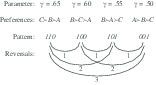
Data are coded so that 000 is the intransitive response pattern of
choosing A over B, B over C, and C
over A. The pattern 111 represents the intransitive cycle of
choosing B over A, C over B, and A
over C. The other six response patterns are transitive.
In Table 4 we see that the participant had perfectly intransitive response
patterns within every single block of the study. The person began with the
intransitive cycle 000 and switched to the opposite intransitive
cycle, 111. Weak stochastic transitivity is violated in the binary
choice proportions, because P(B ≻ A) >
½, P(C ≻ B) >
½ and P(A ≻ C) >
½. Yet the marginal choice proportions (0.6, 0.6, 0.6) are
perfectly consistent with a mixture of linear orders, satisfying the triangle
inequality, P(AB) + P(BC) + P(CA) ≤ 2. If an investigator
analyzed only marginal choice proportions, the conclusion from the triangle
inequality would be that transitivity can be retained. By examining response
patterns, however, it is easy to see that every individual response pattern was
intransitive.
Cha et al. (2013, pp. 66–68) conceded this point, but they claimed
that the TE models would also fail to detect intransitivity in such
cases. However, that claim depends on their assumption that the TE
model satisfies independence, which it does not.
Table 5: Analysis of response patterns from hypothetical data of Table 4.
Response pattern
Observed ABC
Observed
A′B′C′
Observed
both
Predicted ABC (iid)
Predicted both (iid)
000
8
8
8
1.28
.08
001
0
0
0
1.92
.18
010
0
0
0
1.92
.18
011
0
0
0
2.88
.41
100
0
0
0
1.92
.18
101
0
0
0
2.88
.41
110
0
0
0
2.88
.41
111
12
12
12
4.32
.93
Sum
20
20
20
20
2.81
The response patterns from Table 4 are cross-tabulated in Table 5. Table 5
is perfectly consistent with iTET in this case, which can violate
response independence.
Table 5 also shows the response frequencies predicted from the iid model. The
hypothetical data do not satisfy the predictions of iid at all. Among the
predictions of iid, note that if the marginal choice proportions are each 0.6,
the total probability that a response pattern will be repeated within blocks is
only 0.14; so out of 20 trials, the person is expected to agree in choice
pattern only 2.81 times within blocks. In these hypothetical data, however,
the participants were perfectly consistent (20 agreements = 100%). Do real
data show higher self-consistency than predicted by independence? They do
(Birnbaum & Bahra, 2012a, Footnote 4; Birnbaum & Bahra, 2012b, Appendix H).
The examples in Birnbaum (2012a), like that in Table 5, are cases
where the cross-tabulations are perfectly consistent with TE models
and error rates are zero. Perhaps these perfect features of the
examples led Cha et al. (2013, p. 70) to state that, if TE models
are allowed to violate iid, they always fit perfectly and are
therefore not testable. The next sections show the appropriate TE
models for testing transitivity in the presence of error, and
illustrate cases where the TE model leads to different conclusions
from those reached by the methods used by Regenwetter et al. (2011).
Examples where TE models can be rejected are also presented.
3.2 True-and-error model for Test of Transitivity
There are 8 possible response patterns for each test with three choice
problems testing transitivity: 000, 001, 010,
011, 100, 101, 110, and 111. In
the TE model, the predicted probability of showing the intransitive pattern,
111, is given as follows:
P(111) =
p000(e1)(e2)(e3)
+
p001(e1)(e2)(1
– e3)
+ p010(e1)(1 –
e2)(e3) +
p011(e1)(1 –
e2)(1 – e3)
+ p100(1 –
e1)(e2)(e3)
+ p101(1 –
e1)(e2)(1 –
e3)
+ p110(1 – e1)(1 –
e2)(e3)
+ p111(1 – e1)(1 –
e2)(1 – e3). (4)
P(111) is the theoretical probability of observing the
intransitive response cycle of 111;
p000,
p001,
p010, p011,
p100, p101,
p110, and p111 are
the probabilities that the person has these “true” preference patterns,
respectively (these 8 terms sum to 1); e1,
e2, and e3 are the
probabilities of error on the AB, BC, and CA
choices, respectively. These error rates are assumed to be mutually
independent, and each is less than ½.
There are seven other equations like Equation 4 for the probabilities of the
other seven possible response patterns.
Because each choice is presented twice in each block, there are 64 possible
response patterns for all six responses within each block. If error rates are
assumed to be the same for choice problems A′B′, B′C′, and
C′A′ as for choice problems AB, BC, and CA,
respectively, the probability of showing the same pattern, 111, on
both versions in a block is the same as in Equation 4, except each of the error
terms, e or (1 – e) in Equation 4 are squared. In this way,
one can write out 64 expressions for all 64 possible response patterns that can
occur in one block.
Table 6: Hypothetical data containing error that illustrate testing
independence, TE model, and transitivity. Analyses described in the text show
that these data violate independence, they satisfy TE model, and they violate
transitivity.
Response Pattern in A′B′C′ choices
ABC
000
001
010
011
100
101
110
111
Sum
000
17
3
4
1
6
1
2
2
36
001
3
1
1
1
1
1
0
1
9
010
5
1
0
1
2
1
1
2
13
011
1
1
1
3
1
3
2
11
23
100
6
1
2
1
2
0
1
2
15
101
1
1
1
3
1
2
2
8
19
110
2
0
1
2
1
2
2
6
16
111
1
1
3
11
2
9
6
36
69
Sum
36
9
13
23
16
19
16
68
200
A hypothetical set of data is shown in Table 6. The rows show the 8 possible
response combinations for the ABC choices and the columns show the 8
possible response patterns for the A′B′C′ choices. Each entry is the
frequency with which each response pattern occurred. For example, the 17 in
the first row and column shows that on 17 out of 200 blocks, the person showed
the intransitive pattern, 000, in both versions of the three choice
problems.
The general TE model for this case has 8 parameters for the 8
“true” probabilities and 3 error rates (one for each choice
problem).4 Because these 8 “true”
probabilities sum to 1, they use 7 df, so the model uses 10 df to
account for 64 frequencies of response patterns; the data have 63 df
because they sum to the total number of blocks. It should be clear
that there are many ways for 64 frequencies to occur that are not
compatible with a model with 11 parameters. Two examples will be
presented later.
The transitive TE model is a special case of this general TE model
in which the two probabilities of intransitive patterns are set to zero,
p000 = p111
= 0. If the error rates are not zero, a set of data can (and typically would)
still show some instances of intransitive response patterns, even though the
“true” probabilities of these patterns are each zero.
One can conduct at least three types of statistical tests. First, one
can test independence. Second, one can test this general TE model.
Third, if the general TE model provides a reasonable approximation,
one can test the special case of transitivity within that
model.5
According to response independence, it should be possible reproduce the
entries in Table 6 from just three numbers: the marginal choice proportions,
P(AB), P(BC), and P(CA).
These are all 0.6, so the predicted entry for the upper left cell of Table 6
(000, 000) would be [1 –
P(AB)]2[1 –
P(BC)]2[1 –
P(CA)]2 = (.4)6 = 0.004.
Multiplying by the total frequency (200), the predicted frequency is 0.82, far
less than the observed value of 17.
For an overall index of fit, one can compute
χ2 =
Σ(fi –
Fi)
2/Fi. Where
fi are the observed frequencies and
Fi are the corresponding predicted
frequencies, based on independence (or below, predicted from the TE
model). There are 63 df in the data, and we used 3 df to estimate the
three parameters (the marginal choice proportions), so this test of
independence has 60 df. In this case, χ2(60)
= 505.4, so the conclusion would be that these data do not satisfy
response independence.6
Next, one can use a function minimizer, such as the solver in Excel, to
estimate best-fit parameters for the general TE model. Those estimates are
p000 = .333,
p111 = .667,
p001 = p010
= p011=
p100 =
p101=
p110 = 0; e1 = 0.25,
e2 = 0.20, and e3 = 0.15. In
this case, 10 df were used to estimate the parameters, and
χ2(53) = 11.5, showing that the general TE model fits
these hypothetical data well.
However, when we fix p000= p111 = 0, in order to test the transitive
special case, and solve for the best-fit parameters, we find that the
transitive TE model does not fit these data, χ2(55) =
108.3. The difference, χ2(2) = 108.3 – 11.5 = 96.8,
indicates that transitivity is not satisfactory as a description of these same
data.
These calculations show that, in principle, one can estimate the models and
assess their fit in the 8 × 8 matrix as in Table 6. In practice, however, it
might be difficult or impractical to obtain sufficient data for such a full
analysis. When the data are thinner, one might partition the data in various
ways and still test independence, TE model, and transitivity, as described
next.
3.3 Partitions of the data
Table 7: Hypothetical examples testing transitivity; these examples illustrate
use of partitioned data to compensate for small sample sizes. Marginal choice
proportions are the same in all examples. Examples 1-3 violate iid. Example 1
satisfies transitivity, which is violated in Examples 2 or 3. Frequencies under
“ABC” represent response patterns to Choice AB,
BC, and CA, so 000 and 111 are intransitive; frequencies
under “Both” indicate the same response pattern repeated within blocks.
Example 4 satisfies iid model of Regenwetter et al. (2011), which wrongly
concludes that all four of these examples satisfy transitivity.
Pattern
Example 1
Example 2
Example 3
Example 4
ABC
Both
ABC
Both
ABC
Both
ABC
Both
000
2
0
27
20
11
7
6
0
001
5
1
4
0
4
0
10
1
010
5
0
4
0
4
0
10
1
011
28
20
5
1
21
14
14
2
100
13
7
4
0
20
13
10
1
101
20
13
5
1
5
0
14
2
110
20
13
5
0
5
1
14
2
111
7
1
46
33
30
20
22
5
Total
100
55
100
55
100
55
100
14
χ2 Indep
335.18
1139.25
408.95
0.52
In order to test independence to compare the iid models with TE models, one
might partition the data from the 8 × 8 matrix (as in Table 6) into three, 2 ×
2 matrices, in order to test the models of repetitions, as was done in Tables 2
and 3. For example, one can tabulate the AB choice by the
A′B′ choice. From Table 6, the four frequencies are 44, 37, 37, and
82, for 00, 01, 10, and 11, respectively. These violate independence by a
standard chi-square test, χ2(1) = 10.8. However, the
same values fit the TE model, χ2(1) = 0.2, with
e1 = 0.25. Similarly, the tabulations for the other
two choice problems also violate response independence,
χ2(1) = 20.7 and 40.3, and also satisfy TE
independence, χ2(1) = 0.1, and 0.5, with
e2 = 0.2, and e3 = 0.15,
respectively. Because these error estimates do not assume or imply the property
of transitivity, they might be used to constrain solutions to other partitions
of the data that can be used to test transitivity.
A useful partition for testing transitivity is to count the frequencies of
the 8 possible response patterns in the AB, BC, and
CA choices and the frequencies of repeating the same patterns on both
ABC and A′B′C′ choices within blocks. These values can be
found in the row sums of Table 6 and on the major diagonal, respectively. But
these frequencies contain cases in common, so they are not mutually exclusive.
One can construct a mutually exclusive, exhaustive partition by counting the
frequency of showing each pattern on both repetitions of the same choice
problems and the frequency of showing each of 8 response patterns in the
ABC choices and not in both cases. For example, in Table 6, the
frequency of showing the 000 pattern in the ABC choice problems and
not in both forms is 36–17 = 19.
This partition of the data reduces the 64 cells as in Table 6 to 16 cells.
This partition has the effect of increasing the frequencies in each cell, but
reducing the degrees of freedom in the test. In this partition, we can also
test independence, TE model, and transitivity. The purpose of the partition is
to increase the frequencies within each cell, in order to meet the assumptions
of the Chi-Square or G-Square statistical tests.
Four examples of hypothetical data are shown in Table 7 to illustrate different
cases that might be observed with this type of partition. The numbers have
been chosen to sum to 100 so that they could be easily converted to proportions
to facilitate calculations for the models.
All four examples in Table 7 have identical marginal choice proportions, so
any method of analysis that focused strictly on marginal choice proportions
treats these four examples as identical, but they are quite different from each
other. The marginal choice proportions, P(AB),
P(BC), and P(CA) are all 0.6, so these
examples all violate weak stochastic transitivity, and all satisfy the triangle
inequality. However, they have different interpretations, as shown below.
These response patterns are listed in terms of the ABC choice
pattern and repeated patterns. To convert to a mutually exclusive and
exhaustive partition, subtract the “both” frequencies from the ABC
frequencies, as described above. The Chi-Squares are then computed in the
conventional way comparing observed frequencies with those predicted by the
models.
First, we can test independence, which is the assumption that products of
marginal choice proportions correctly reproduce all 16 cells in this partition
of the data. Three parameters (three marginal choice proportions) are
calculated from the data, leaving 15 – 3 = 12 df for the test of independence.
The critical value of χ2(12) with α = .01 is
26.22. The last row of Table 6 shows these χ2 tests;
only Example 4 satisfies independence.
Second, we can test the general TE model. The TE model can also be tested by
this partition because there are 15 df in the data and the model uses 7 df for
the 8 “true” probabilities and 3 df for the three error rates
(e1, e2, and
e3 for Choices AB, BC, and
CA, respectively). That leaves 5 df to test the model in this
partition.7
Table 8: Best-fit solutions of TE models to Example 2 of Table 7. These
hypothetical data satisfy the triangle inequality yet are perfectly
intransitive, according to the fit of the TE models. Fixed values are shown in
parentheses and constrained values are shown in brackets. Constrained errors
are estimated strictly from preference reversals to the same choice problem
within blocks, using the three, 2 × 2 partitions as in Table 3.
Unconstrained errors
Constrained errors
Parameter
General
Transitive
Intransitive
General
Transitive
Intransitive
p000
0.378
(0)
0.378
0.378
(0)
0.375
p001
0.000
0.342
(0)
0.000
0.141
(0)
p010
0.000
0.045
(0)
0.000
0.116
(0)
p011
0.011
0.000
(0)
0.011
0.184
(0)
p100
0.000
0.030
(0)
0.000
0.116
(0)
p101
0.011
0.015
(0)
0.011
0.184
(0)
p110
0.000
0.568
(0)
0.000
0.259
(0)
p111
0.600
(0)
0.622
0.601
(0)
0.625
e1
0.095
0.024
0.112
[0.1]
[0.1]
[0.1]
e2
0.095
0.024
0.112
[0.1]
[0.1]
[0.1]
e3
0.103
0.500
0.091
[0.1]
[0.1]
[0.1]
χ2
1.98
88.48
3.29
2.02
4194.97
3.67
Third, if the TE model fits, we can test the transitive model by fixing the
values of p000 =
p111 = 0, which means that the solution is
restricted to be purely transitive. The difference in fit between the general
case where probabilities of all “true” patterns are free and the transitive
special case provides a test of transitivity on 2 df.
Example 1 of Table 7 violates independence [χ2(12)
= 335.18]; however, it satisfies both the TE model and transitivity. The TE
model fit these data with error rates constrained to match the preference
reversals data only, where e1 =
e2 = e3 = 0.1, where
p000 = p111 = 0 were fixed,
and where the best-fit solution yielded p001
= 0, p010 = 0,
p011 = 0.325,
p100 = 0.125,
p101 = 0.25, and
p110 = 0.25. This model has
χ2 = 2.04, so it should be clear that there is no room
for a significant improvement by making the model more complex. So this case
violates iid, but satisfies the TE model and transitivity.
However, Example 2 is a very different case from Example 1, as shown in
Table 8. Six models have been fit to those data, including the general TE
model (all 8 response patterns allowed), the transitive special case (both
intransitive patterns are fixed to zero), and a purely intransitive model (only
intransitive patterns are allowed). Parameters shown in parentheses are fixed,
and those shown in square brackets are constrained.
When the general TE model fits the data, one might constrain the error
rates in this analysis to agree with values estimated strictly from
replications data (from the three, 2 × 2 cross-tabs). The constrained version
provides greater power for the test of transitivity.
The fact that the TE general model fits either with or without constrained
errors shows that we can retain the general TE model. The differences in
Chi-Squares between the general model and the transitive special case are large
enough to reject the transitive model either with or without constrained errors
(χ2(2) = 4192.95 and 86.50, respectively). The purely
intransitive special case also fits these data acceptably because the
difference in Chi-Squares between the general model and purely intransitive
model is not significant in either constrained or free cases.
Table 9: Fit of TE models to Example 3 of Table 7. These hypothetical data
satisfy the triangle inequality but they contain a mixture of transitive and
intransitive response patterns. Neither the purely transitive nor purely
intransitive solutions yields an acceptable fit.
Unconstrained errors
Constrained errors
Parameter
General
Transitive
Intransitive
General
Transitive
Intransitive
p000
0.128
(0)
0.406
0.128
(0)
0.476
p001
0.000
0.000
(0)
0.000
0.000
(0)
p010
0.000
0.001
(0)
0.000
0.000
(0)
p011
0.255
0.597
(0)
0.256
0.520
(0)
p100
0.242
0.360
(0)
0.243
0.257
(0)
p101
0.000
0.000
(0)
0.000
0.130
(0)
p110
0.011
0.042
(0)
0.011
0.093
(0)
p111
0.363
(0)
0.594
0.364
(0)
0.524
e1
0.101
0.500
0.493
[0.1]
[0.1]
[0.1]
e2
0.104
0.107
0.000
[0.1]
[0.1]
[0.1]
e3
0.090
0.000
0.142
[0.1]
[0.1]
[0.1]
χ2
1.66
23.32
27.22
1.69
1067.77
1069.16
Table 9 shows the corresponding analyses for Example 3. The general TE model
is again acceptable with or without constrained errors. In this case, however,
both the purely transitive model and the purely intransitive model can be
rejected. Therefore, one would conclude that these data are best represented
as a mixture of transitive and intransitive response patterns.
Example 4 satisfies independence. In that case, one could say that the data
might be compatible with a mixture of strictly transitive patterns, but one
might also say that the data could have arisen from a mixture that included
intransitive patterns. In the analyses of Regenwetter et al. (2011), this
case would be declared consistent with transitivity, as would all of these
examples. In the approach of Regenwetter et al. (2011), no statistical test
would be conducted because the model “fits perfectly” in all of these cases.
Table 10: Hypothetical examples violating both response independence and the TE
model with all parameters free. As in Table 7, these examples have the same
marginal choice proportions (all 0.6).
Example 5
Example 6
Pattern
ABC
Both
ABC
Both
000
28
4
1
0
001
4
0
1
0
010
4
0
1
1
011
4
0
37
4
100
4
0
19
4
101
4
0
19
4
110
4
0
19
4
111
48
6
3
1
Total
100
10
100
18
χ2 Indep
156.5
93.1
χ2 TE
84.8
69.8
Table 10 provides two hypothetical examples showing that the TE model need not
always fit. Marginal choice proportions in Examples 5 and 6 are the same as in
Examples 1–4 of Table 7. In both cases iid is violated, but in both cases the
general TE model fails. In Example 5, the response patterns observed are mostly
intransitive and in Example 6 most of the response patterns observed are
transitive.
To understand what went wrong for the TE models in these examples, recall that
errors are assumed to be mutually independent. Although TE models violate
independence of responses, they satisfy independence of errors, and the errors
in these examples violate that assumption. In these examples, the participant
was not completely consistent so errors are not zero; we know that there are
substantial errors because people did not repeat the same response patterns in
both versions very often. But if errors are not zero and are mutually
independent, we should have observed more instances of response patterns 001,
010, 100, 011, 100, 101, and 110 in Example 5, and yet too few such cases are
observed. Instead, whenever a person made an error on one choice problem, they
too often made an error on other choice problems. Example 6 also violates TE
because data violate independence of errors. Examples 5 and 6 violate iid and
violate TE model.
In summary, one can separately test independence, TE, and transitivity.
These examples illustrate how the TE model can be applied and they refute the
claims by Cha et al. (2013) that TE models must satisfy response independence
or become vacuous.
Difficulties in the approach of Regenwetter et al. (2011) are illustrated by
these examples. Based on marginal choice proportions, all of these examples
are the same and all are perfectly consistent with transitivity. When we
examine the data as in Tables 6-10, we see that some cases systematically
violate iid and among those, some cases systematically violate transitivity and
others satisfy it. When iid assumptions are satisfied, then marginal choice
proportions contain all of the useable information in the data, but when iid is
violated, we need to examine response patterns to correctly diagnose the
substantive issue of transitivity.
These hypothetical examples illustrate why it is important to know whether iid
assumptions, especially response independence, are empirically satisfied in
choice experiments. Birnbaum and Bahra (2007b, 2012b) found that iid was
violated in a series of experiments testing transitivity. Birnbaum’s (2012a)
reanalysis of Regenwetter et al. (2011) also concluded that iid was not
satisfied for those data.
However, Cha et al. (2013) claimed that the findings from Birnbaum (2012a) were
“not replicated within subjects” when other data sets from Regenwetter et
al. (2011) were examined, that the tests proposed have “unknown”
p-values that are significantly different from those obtained by
another method of simulation, and that certain other tests of “iid” were
satisfied “with flying colors” for the Regenwetter et al. (2011) data. Each
of these claims is refuted in Appendix A, where it is shown that the evidence
against iid is significant in all three sets of data reviewed by Cha et al.,
that the p-values estimated by Birnbaum’s methods are conservative
relative to the method used by Cha et al., and that the tests of “iid” that
were not significant “with flying colors” in Cha et al. do not test response
independence.
3.4 Birnbaum and Bahra data violate iid
Birnbaum and Bahra (2007b, 2012b) also used three designs for each
participant in each study; they used 136 participants (in three studies)
compared to 18 in Regenwetter et al. (2011) and they asked each person to
respond twice to each choice problem in each block (compared to once per block
in Regenwetter et al., 2011). They also used a greater variety of choice
problems that might be expected to create more interference in memory, and
blocks were properly separated by numerous intervening tasks. Therefore, this
2012b paper with 136 participants must be accorded corresponding greater weight
in relation to a study with only 18 participants. As shown in Birnbaum and
Bahra (2012b), evidence against iid in those studies was extremely strong.
Birnbaum and Bahra (2007b, 2012b) found that a number of participants completely
reversed preferences for 20 out of 20 choice problems between blocks; this
provides a clear refutation of the theory of iid. Because each block of each
design in that study contained 20 experimental choice problems (excluding
fillers and separators), a complete reversal has a probability of
½ to the 20th power, assuming iid, which is less
than one in a million. There were 18 people out of 136 who showed at least one
such perfect reversal of 20 out of 20 responses between blocks, and these 18
produced hundreds of instances of such perfect reversals. In fact, one person
reversed preferences perfectly between 60 choice problems (all three designs)
between blocks (see Table 2 of Birnbaum & Bahra, 2012b). These and other
analyses of those data show that iid can be rejected.
4 Discussion
In my opinion, the empirical results obtained so far tell us that any viable
approach to analyzing formal properties in choice data should be able to handle
the possibility that the assumptions of response independence is violated. It
should allow for the possibility that people behave more consistently than
allowed by the simplifying assumptions of iid. The TE models can handle
certain violations of response independence. These models do not satisfy
response independence and yet they are testable because they cannot handle all
such violations.
As shown in the examples presented here, TE model can distinguish and diagnose
cases that look identical to tests defined on marginal choice proportions (such
as weak stochastic transitivity and the triangle inequality). All of the
examples in Tables 6, 7, and 10 have the same binary choice proportions.
However, I think it proper to conclude that Example 1 of Table 7 satisfies
transitivity and that Examples 2 and 3 in Table 7 violate it. Example 4
satisfies iid and is therefore open to debate, because a person might have a
mixture that is purely transitive or might have a mixture including
intransitive patterns and still produce such data.
These different conclusions for these different examples could not be reached by
examination of the marginal choice proportions alone, because they all have the
same marginal proportions. My advice to those testing transitivity or other
properties is that they should analyze data at the level of response patterns
rather than at the level of marginal choice proportions.
4.1 Are criticisms of using marginal proportions dependent on the TE model?
No, these criticisms apply whenever iid is violated, whatever the cause.
The TE models provide one approach, but this family is not the only way that
violations of iid might be represented. The criticism of using only marginal
choice proportions applies to any case in which iid is violated, whether those
violations satisfy a TE model or not. As shown in Examples 5 and 6 of Table
10, data might violate iid and also violate the TE model. These examples,
including those in Table 3, show that the assumption of independence of errors
is a testable property of these models, but it is not the same as response
independence.
One could argue that TE models are only approximate because they allow that
a person can change “true” preferences between blocks but not within a block.
A more accurate or more general model might allow that a person might change
“true” preferences at any point during the study. Such a model would include
the iid model used by Regenwetter et al. (2011) and TE models as special cases.
According to the model used by Regenwetter et al. (2011), independence is
supposed to hold on every experimental trial, as long as there are three filler
trials separating experimental trials.
4.2 What if TE models are wrong or incomplete?
The TE Models are testable and they might be rejected when appropriate
studies have been done. A test of iTET requires a larger quantity of
data from each participant to conduct a proper analysis, whereas tests of
gTET require a large numbers of participants, each of which might
contribute a smaller amount of data. Whereas a number of experiments in the
gTET paradigm have been published, we do not yet have experimental
results comparable to the hypothetical Table 6 for the iTET case, and
one might reasonably wish for even more data than described in that example.
Although TE models can allow different error rates in different choice
problems, and although more general versions can be tested in which different
people might have different amounts of noise in their data, even these more
general TE models do not provide any fundamental explanation for the sources of
the errors.
Nor do TE models proposed so far provide an explanation for the kinds of
sequential effects that might arise from a process such as described by
Birnbaum (2011), in which the parameters of a model of risky decision making
change systematically from trial to trial, as elaborated in Appendix B.
Therefore, although TE models provide a testable framework within which issues
of independence and transitivity can be explored, they do not provide specific
or satisfying answers to important deeper questions. Appendix B shows how
sequential models might account for violations of iid including response
independence as well as violations detected by the correlation test of Birnbaum
(2011, 2012a). These models allow that parameters representing probability
weighting or risk aversion might fluctuate from block to block, but they do not
identify the causes of changing parameter values.
But it is important to realize that even if TE models are wrong, as in
Examples 5 and 6 of Table 9, or if they are approximate, incomplete or even
misguided, criticism of TE models does not mitigate the problems of assuming
iid as a basis for testing transitivity. The key problem is that when iid is
violated, analysis of marginal choice proportions can easily lead to wrong
conclusions.
4.3 Are assumptions of iid only used to justify statistical tests?
It might be argued that because the assumptions of iid are used to justify
statistical tests, that this is their only role in the approach of Regenwetter
et al. (2011). That is not true: in fact, it is the assumption of iid that
justifies analysis of marginal choice proportions. As shown in the examples of
Table 6 and 7, when iid is violated, marginal choice proportions might satisfy
the triangle inequality despite systematic violations of transitivity within
blocks, revealed in the response patterns.
The statistical issue (that violations of iid affect the p-value of a
significance test) is far less important, in my opinion, than the danger of
drawing wrong descriptive, substantive conclusions concerning a theoretical
property (such as transitivity) from marginal choice proportions. Indeed, when
the triangle inequalities are satisfied, as they are in all of the examples
analyzed here, the Regenwetter et al. (2010, 2011) approach conducts no
statistical test at all, because the model is said in all of such cases to fit
“perfectly”. For example, in Table 7 the triangle inequality can be
“perfectly” satisfied in a case in which a different, deeper analysis (Table
8) would refute any mixture of transitive patterns in favor of a mixture of
purely intransitive patterns.
There is another distinction that might be helpful to eliminate some
confusion in this dispute. The random preference model used by Regenwetter et
al. (2011) allows any set of preference patterns to be in the “mind” of the
participant. These hypothesized preference patterns can violate independence.
Indeed, in the linear order, no intransitive patterns are allowed, so it might
seem that this model violates a type of independence in the postulated mental
set.
However, on each trial, the Regenwetter et al. (2011) model assumes that the
choice response can be represented as the result of an independent, random
sample from the collection of mental preference patterns. Because that
“random preference” sampling is random, it means that overt responses will
satisfy independence, even when the theoretical preference patterns in the
hypothesized collection (in the mind) violate independence.
Regenwetter et al. (2011) have pointed out that it is not possible to recover
the distribution of true preference patterns from the choice responses of a
person, because the assumed independence of responses means that overt
responses do not permit recovery of the distribution of preference patterns in
the mind of the participant.
The assumption of response independence thus justifies analysis of marginal
choice proportions, while it also makes it impossible to identify the
distribution of theorized preference patterns. When iid is assumed, one might,
in principle, reject transitivity in this approach, but one cannot recover the
distribution of “true” response patterns in this model nor can one
definitively rule out mixtures containing intransitive response patterns when
the marginal means satisfy transitivity. As shown here, when iid is violated,
satisfaction of the triangle inequality can co-exist with systematic violations
of transitivity.
The statistical tests used here to illustrate analyses in the TE model also make
independence assumptions, but these do not assume nor imply response
independence. Obviously, these higher order assumptions might be empirically
wrong. But if and when the model is appropriate, it can be used to estimate
the distribution of “true” response patterns.
4.4 The details are in the data
The question of how much detail should be analyzed in data arises in all
research problems. The analyses of the various partitions of the data here
should clarify that whenever data are aggregated, information can be lost.
This debate can be viewed as a debate of how much useful information is
contained in data and how much detail should be represented by a model.
For example, there are 20 × 6 = 120 Values in Table 4. In a larger experiment,
there might be a hundred rows. Such a table of data might be summarized by 3
binary choice proportions, by 6 column proportions, by 3, 2 × 2
cross-tabulations of repeated responses, by 8 proportions of showing each
response pattern involving three choice problems, by 8 × 2 proportions showing
each response pattern on the ABC choice (but not both) and in both versions, by
the 8 × 8 cross-tabulation of the eight response patterns in
the ABC × A′B′C′
repetitions, or at the level of the original data.
When response independence is violated, as appears to be the case for all three
sets of data in Regenwetter et al. (2011) as well as the series of studies in
Birnbaum and Bahra (2012b), it means that marginal choice proportions do not
tell the whole story. As shown here, response independence and error
independence are different properties, but both properties can be tested, and I
think it would be a true error not to test them both.
References
Birnbaum, M. H. (2004). Tests of rank-dependent utility and cumulative prospect
theory in gambles represented by natural frequencies: Effects of format, event
framing, and branch splitting. Organizational Behavior and Human
Decision Processes, 95, 40–65.
Birnbaum, M. H. (2008). New paradoxes of risky decision making.
Psychological Review, 115, 463–501.
Birnbaum, M. H. (2011). Testing mixture models of transitive preference: Comment
on Regenwetter, Dana, and Davis-Stober (2011). Psychological Review,
118, 675–683.
Birnbaum, M. H. (2012a). A statistical test of the assumption that repeated
choices are independently and identically distributed. Judgment and
Decision Making, 7, 97–109.
Birnbaum, M. H. (2012b). True and error models of response variation in judgment
and decision tasks. Workshop on Noise and Imprecision in Individual and
Interactive Decision-Making, University of Warwick, U.K., April, 2012.
Birnbaum, M. H., & Bahra, J. P. (2007a). Gain-loss separability and coalescing
in risky decision making. Management Science, 53, 1016–1028.
Birnbaum, M. H., & Bahra, J. P. (2007b). Transitivity of preference in
individuals. Society for Mathematical Psychology Meetings, Costa Mesa,
CA. July 28, 2007.
Birnbaum, M. H., & Bahra, J. P. (2012a). Separating response variability from
structural inconsistency to test models of risky decision making.
Judgment and Decision Making, 7, 402–426.
Birnbaum, M. H., & Bahra, J. P. (2012b). Testing transitivity of preferences in
individuals using linked designs. Judgment and Decision Making, 7,
524-567.
Birnbaum, M. H., & Gutierrez, R. J. (2007). Testing for intransitivity of
preference predicted by a lexicographic semiorder. Organizational
Behavior and Human Decision Processes, 104, 97–112.
Birnbaum, M. H., & LaCroix, A. R. (2008). Dimension integration: Testing models
without trade-offs. Organizational Behavior and Human Decision
Processes, 105, 122–133.
Birnbaum, M. H., & Schmidt, U. (2008). An experimental investigation of
violations of transitivity in choice under uncertainty. Journal of Risk
and Uncertainty, 37, 77–91.
Birnbaum, M. H., & Schmidt, U. (2012). Constant consequence paradoxes of
Allais: Coalescing, restricted branch independence, or error?
Foundations of Utility and Risk XV (FUR XV), Atlanta, July, 2012.
Carbone, E., & Hey, J. D. (2000). Which error story is best? Journal of
Risk and Uncertainty, 20, 161–176.
Cha, Y., Choi, M., Guo, Y., Regenwetter, M., & Zwilling, C. (2013). Reply:
Birnbaum’s (2012) statistical tests of independence have unknown Type-I error
rates and do not replicate within participant. Judgment and Decision
Making, 8, 55–73.
Conlisk, J. (1989). Three variants on the Allais example. American
Economic Review, 79, 392–407.
Harless, D. W., & Camerer, C. F. (1994). The predictive utility of generalized
expected utility theories. Econometrica, 62, 1251–1289.
Lichtenstein, S., & Slovic, P. (1971). Reversals of preference between bids
and choices in gambling decisions. Journal of Experimental Psychology,
89, 46–55.
Loomes, G., & Sugden, R. (1998). Testing different stochastic specifications
of risky choice. Economica, 65, 581–598.
Loomes, G., Starmer, C., & Sugden, R. (1991). Observing violations of
transitivity by experimental methods. Econometrica, 59, 425–439.
Regenwetter, M., Dana, J. & Davis-Stober, C. (2010). Testing transitivity of
preferences on two- alternative forced choice data. Frontiers in
Psychology, 1, 148. http://dx.doi.org/10.3389/fpsyg.2010.00148.
Regenwetter, M., Dana, J., & Davis-Stober, C. P. (2011). Transitivity of
preferences. Psychological Review, 118, 42–56.
Regenwetter, M., Dana, J., Davis-Stober, C. P., and Guo, Y. (2011).
Parsimonious testing of transitive or intransitive preferences: Reply to
Birnbaum (2011). Psychological Review, 118, 684–688.
Smith, J. B., & Batchelder, W. H. (2008). Assessing individual differences in
categorical data. Psychonomic Bulletin & Review, 15,
713-731. http://dx.doi.org/10.3758/PBR.15.4.713.
Sopher, B., & Gigliotti, G. (1993). Intransitive cycles: Rational choice or
random error? An answer based on estimation of error rates with experimental
data. Theory and Decision, 35, 311–336.
Tversky, A. (1969). Intransitivity of preferences. Psychological Review,
76, 31–48.
Wilcox, N. T. (2008). Stochastic models for binary discrete choice under risk:
A critical primer and econometric comparison. Research in Experimental
Economics, 12, 197–292.
Appendix A: Additional data, simulations, and reanalyses
Other Data of Regenwetter et al. (2011)
Birnbaum (2012a) analyzed only that part of the study of Regenwetter
et al. (2011) that replicated Tversky’s (1969) study, called “Cash
1.” Cha et al. (2013) claimed that when two other sets of data from
that study, “Cash 2” and “Noncash”, which used different stimuli,
are examined, Birnbaum’s tests were “not replicated within subjects”
and when other statistics were computed, that iid was satisfied “with
flying colors”. However, when I reviewed all three sets of data, I
do not concur with their conclusions.
According to iid, there should be no correlation between the number of
preference reversals between two blocks and the separation between blocks. If
observed correlation coefficients differ from zero, we expect half to be
positive and half negative, if iid holds. Birnbaum (2012a) previously reported
that 15 of 18 participants had positive correlations in Cash 1, that the median
correlation was 0.58, and that the mean correlation was significantly greater
than zero by a conventional t-test.
When these correlations are calculated for Cash 2 and Noncash conditions, 12 and
15 of the 18 correlation coefficients are greater than zero, respectively; the
median correlation coefficients were 0.39 and 0.63, respectively. Mean
correlations were significantly greater than zero by t-tests in both
Cash 2 and Noncash (t(17) = 3.21 and 5.00, respectively). Across all
three sets of data, 42 of 54 correlation coefficients (3 data sets by 18
participants) are greater than zero, which is significantly more than half
(binomial p = .00003). The overall median correlation was 0.51, which
seems substantial.
I conclude that adding Cash 2 and Noncash datasets makes the case against iid
even stronger than it was without them, even when conventional statistics are
applied. The evidence against iid was indeed “replicated” in a “within
subjects design” if these terms are interpreted as finding a significant test
statistic with new stimuli in tests with the same participants.
Simulated p-values
Cha et al. (2013, Table 5, left side) presented the results of 108 statistical
tests of iid for the Regenwetter et al. (2011) data. They used Birnbaum’s
(2012a) R-program to simulate two statistical tests for each of 18 participants
in three sets of data with 10,000 random simulations per data set.
Separating the tests by data sets, there were 9, 11, and 9 “significant”
violations (p < 0.05) in Cash 1, Cash 2, and Noncash
conditions, respectively. For the correlation test alone, 5 out of 18 were
significant in each of the three conditions. The binomial probability to
observe five or more significant results out of 18 with p = .05 is
.0015, so each condition provides significant refutations of iid taken alone.
Similarly, there were 4, 6, and 4 who violated the variance test in the three
conditions. The binomial probability to observe 4 or more with p =
.05 is .011, so iid can be rejected separately in all three conditions for this
test as well. Thus, all six tests are significant: 3 data sets by 2 tests per
data set.
Given the lack of power—there are only 18 participants who responded to each
choice only 20 times—these findings seem strong evidence against iid.
Summing across participants, data sets, and tests, Cha et al. reported that 29
of 108 tests were “significant” with p < .05, using
Birnbaum’s algorithm.
Suppose we adopted the following extra-conservative standard: Suppose we
required the simulated p-value to be .02 or less in order to
conclude it is actually “significant” at .05. According to Table 5 of Cha et
al, there are 25 such values. According to the binomial distribution with
n = 108 and p = .05, the probability to observe 25 or more
“significant” tests, if the null hypothesis is true, is less than one in a
billion. So, despite using a doubly conservative procedure to evaluate the
significance tests, these data say we should reject the hypothesis that these
participants are a random sample of people who satisfy iid beyond all
conventional significance levels.
The claim that the tests “Do not replicate”
Although the data show overwhelming evidence to refute iid in all
three sets of data with the same participants, Cha et al. (2013, pp.
62–64) made a very unusual argument, claiming that the statistical
tests “do not replicate within participant” (p. 55). They do not
spell out their logic clearly because strong evidence against iid was
obtained in the same group of people in all three subsets of data,
which I would interpret to say that the significant violations of iid
were indeed “replicated” when the same participants were tested with
different stimuli.
It might be argued that if a person had nonsignificant violations, we
should conclude that this same person actually satisfies iid that if a
person has nonsignificant violations of iid with one set of stimuli that this
same individual should never show a significant violation of iid with any other
stimuli. But that requires us to infer that a nonsignificant result means that
the null hypothesis is true and it requires us to generalize this null
hypothesis from one set of stimuli to all other stimuli. Or it might be argued
that if a test is significant for one person with one set of stimuli,
then it should also be significant in any new test with new stimuli. But that
argument would also be specious.
If either of these principles is intended to justify the statement that the
results “did not replicate,” I find these arguments unreasonable. Recall
that Regenwetter et al. (2011b) argued that it would take very large samples
to test iid, and Birnbaum’s (2012a) tests were devised to address the need to
test iid in small samples. With such small samples (low power), it seems best
not to expect every test to be significant even if the null hypothesis were
false for all persons and all sets of stimuli.
Only 5 of 18 participants of Regenwetter et al. (2011) did not show
at least one “significant” violation of iid, according to Table 5 of
Cha et al. (2013). Does that mean that those five nonsignificant
cases actually satisfy iid? I do not think so. Nor do I think we
should conclude that there are no individual differences with respect
to violating iid. I suspect that iid is false for all participants,
but I think we should withhold judgment until there are better data
before deciding whether iid is violated for all persons or just for
some of them.
Comparing methods for simulation of p-levels
To investigate Birnbaum’s (2012a) suggested statistical tests of iid,
Cha et al. (2013, pp. 59–62) conducted 3,000 simulations for three
of their participants. They used a computer program to simulate data,
based on the assumption that the estimated parameters for each person
were the population values. Their simulations were created via a
program that is expected (but not guaranteed) to produce the same
marginal proportions and expected (but not guaranteed) to satisfy iid.
For each of these 3,000 simulations, they then used Birnbaum’s (2012a)
program to create 10,000 simulated permutations of the simulated data.
They reported that the percentage of Type I errors in their simulated
data (which they called the “actual”) were close to the values
simulated by Birnbaum’s (2012a) two tests, although they found some
small differences, including some statistically significant ones,
where Birnbaum’s tests were conservative relative to theirs.
Examining their findings, I conclude that these two methods for simulating Type
I errors are fairly close in agreement, despite some small differences. For
example, Table 4 of Cha et al. (2013) shows that what they call “actual”
(more accurately, simulated) percentages ranged from .7% to 1.4% for 3,000
samples at the “nominal” 1% level (as simulated by Birnbaum’s methods).
“Actual” (simulated from 3,000 samples) data showed 4.2% to 5.6%
violations corresponding to Birnbaum’s nominal (simulation) at 5%. Their
results showed that the two methods for simulating p-levels are
highly correlated and in fairly close agreement, despite small differences such
as one might expect when comparing these two, slightly different methods for
simulating data using pseudo random numbers generated by computer programs.
New simulations
Although they argued (implicitly) that they had a good method for simulating
data, Cha et al. (2013) did not simulate Type I errors for all of the data.
Instead, they used their method only to compare the estimates of
p-values by two procedures for a few cases. Their method samples
independently from binomials whereas Birnbaum’s method used random
permutations, as in Smith and Batchelder (2008).
In order to simulate data by the method used by Cha et al. (2013), find the
line in Birnbaum’s (2012a) code as follows:
for (jj in 1:nchoices) {xperm[,jj] <-- x[sample(nreps,nreps),jj]} }
and change it to the following:
for (jj in 1:nchoices) {xperm[,jj] <-- x[sample(nreps,nreps, replace =
TRUE),jj]} }
No other changes to the program are necessary. With this revision, each datum
is randomly drawn from a binomial population with probability equal to the
marginal choice proportion in the original data, but each new sample need not
have the same marginal choice proportions as in the original data.
Out of 108 simulations (18 subjects × 3 data sets × 2
tests), each based on 10,000 computer generated samples, I found that
29 simulated Type I errors had p < .05 by either
simulation method; two new cases became “significant” and two other
cases that were “significant” by the permutation method dropped to
non-significant. However, the estimated p-values were
smaller in 78 cases for the sampling method and smaller in 22 cases
for the permutation method, with 8 cases the same. Thus, the
permutation method used by Smith and Batchelder (2008, p. 731) and
implemented by Birnbaum (2012a) is conservative relative to
the method that allows the marginal proportions to vary across
samples.
A reason that Birnbaum’s simulations look “conservative” compared to those of
Cha et al. (2013), is apparently that the method used by those authors allows
simulated proportions not to match the proportions in the original data, which
means that it is possible to have samples for a “variable” with all
0s or all 1s in a column; in those samples, that so-called
“variable” becomes a constant, which will be independent of all other
variables and show no sequential effects. That allows iid to fit such simulated
samples better than it would with the permutation algorithm, so the original
data appear more rare (improbable) in comparison. Personally, I prefer the
more conservative, permutation method (which constrains the marginal
proportions to match those in the original data); however, for these data,
these two methods do not produce any material difference to the conclusions.
Combining all three datasets
The tests applied separately to each design are designed to assess whether or
not the assumption of iid is satisfied for trials that are separated by three
intervening trials, as theorized by Regenwetter et al. (2011).
Table 11: Simulations of combined data from Regenwetter et al. (2011). Each
data array is 20 × 30, Repetitions by Choice Problems. Mean = average number
of preference reversals between blocks, var = variance of preference reversals;
r = correlation between mean number of preference reversals and
difference in trial blocks; pV and
pr = estimated p-values for
variance and correlation tests, respectively, based on 10,000 simulations.
Case
mean
var
pV
r
pr
1
9.70
10.03
0.39
0.88
0.00
2
4.75
8.70
0.00
0.91
0.00
3
2.04
1.44
0.62
0.67
0.18
4
5.44
6.53
0.00
0.33
0.50
5
3.48
10.36
0.00
-0.24
0.72
6
7.24
9.77
0.00
0.91
0.00
7
4.96
8.14
0.00
0.94
0.00
8
3.87
5.04
0.00
0.93
0.00
9
10.71
11.56
0.40
0.92
0.00
10
2.78
4.27
0.01
0.50
0.46
11
1.43
1.16
0.42
0.02
0.98
12
8.89
9.17
0.22
0.48
0.21
13
11.78
14.22
0.03
0.76
0.00
14
0.47
0.34
0.52
0.61
0.40
15
6.79
8.62
0.00
0.62
0.08
16
4.55
7.02
0.00
0.89
0.00
17
8.64
8.07
0.62
0.70
0.03
18
9.20
8.86
0.55
0.55
0.13
Cha et al. (2013, p. 64) reasoned that, if iid assumptions were
false, iid would be more likely to fail if all of the choice problems
were analyzed together. To check this possibility, I combined all
three designs, producing a 20 (Reps) × 30 (Choice problems)
array for each person. When these are analyzed using the Monte Carlo
method sampling procedure, 10 and 9 participants had significant
violations of iid at the 0.05 level for the variance and correlation
tests, respectively, and only 5 participants did not have at least one
significant violation. The median correlation between preference
reversals and distance between blocks increased to 0.68, and all
correlation coefficients except one (out of 18) were positive. The
results are shown in Table 11. Similar results were obtained with the
more conservative, permutation method, with the same 5 individuals
lacking a significant violation.
The tests that “passed with flying colors” do not test independence
Cha et al. (2013, p. 59) performed statistical tests on each column
of data separately, which failed to show statistical significance
“with flying colors”. These tests do not assess response
independence, and so these tests do not address the main issue of this
debate, which is that the assumption of response independence could
lead to wrong conclusions in a test of transitivity, as in Tables 6,
7, and 10. Violations of stationarity can produce violations of
response independence (Birnbaum, 2012a, p. 104), however, which would
be the main reason to test stationarity in this debate.
To understand why separate tests of each choice problem (each column) are not
relevant to the issue of response independence, consider a debate between two
researchers concerning whether X and Y are or are not
positively correlated. Researcher 1 computes the correlation coefficient and
finds that it is significant and positive; indeed, a scatterplot of data shows
that as X increases, the conditional mean of Y given
X also increases systematically. Researcher 2 then examines the
distribution of X and the distribution of Y separately (but
not the joint distribution), and declares that tests of iid were satisfied.
It should be fairly obvious that one cannot analyze independence of
columns by analyzing each column separately. Clearly, Cha et al.
(2013) must not have meant to say that iid was satisfied (based on
finding a null hypothesis “with flying colors” for each column
separately), because that would be like a person examining X
and Y separately and saying they are “independent,” without
actually computing a correlation coefficient or examining the
scatterplot of X and Y. Appendix C describes how the
violation of response independence creates covariance that results in
greater variance of preference reversals than allowed by iid in
Birnbaum’s (2012a) tests.
Appendix B: Stochastic process TE models
As noted in Birnbaum (2011, 2012a), results with the correlation test
indicate that there are fewer preference reversals between two blocks of trials
that occur closer together in time than between two blocks that are farther
apart in time. This suggests that people are not randomly and independently
choosing a true pattern of responses in each block of trials but instead that
the true patterns in successive blocks are more similar. Birnbaum (2011, p.
680-681) suggested that such results might be compatible with a process model
in which there are systematic changes of the parameters of a model of risky
decision-making, such as the TAX model (Birnbaum, 2008). Such a systematic
drift in the value of a parameter might result from a deterministic process or
from a stochastic process in which the value of a parameter at time t
is likely to persist at time t + 1.
To illustrate one such process model, consider two-branch gambles of the
form G = (x, p; y), representing a gamble with a
probability of p to win $x and otherwise win $y,
where x > y ≥ 0. Suppose there are three
gambles as follows: A = (100, .50; 0), B = (92, .58; 0) and
C = (84, .66; 0). Suppose that a person’s choices are governed by the
following TAX model for such gambles:
U(G) =
au(x) +
bu(y)
a +
b
(5)
where a = pγ(1–δ/3) and
b = (1–p) γ +
pγ δ /3, and
U(G) is the utility of the gamble. For American
undergraduates with cash prizes ranging from $0 to $150, it has been found
that one can approximate modal choices with u(x) =
x, δ = 1, and with γ between 0 and 1. Assume that a
person chooses gamble G over gamble F if and only if
U(G) > U(F); models satisfying
this assumption are transitive.
Figure 1: Let A = ($100, 0.5; $0), B = ($92,
0.58; $0), and C = ($84, 0.66; $0). Four “true”
preference patterns for Choices AB, BC, and
CA can occur in the TAX model, as the parameter,
γ, varies from 0.65 to 0.50, where the other parameters
are fixed to conventional values: 110, 100,
101, and 001. In the absence of error, the
number of preference reversals between these patterns varies from
0, when the person retains the same true preferences, to 3 out of
3, when this person’s γ changes from 0.65 to 0.5.
Figure 1 illustrates the four true preference patterns possible for
plausible values of γ. In the case of the gTET
model, one might assume that there are four different types of
participants, with different values of γ. In the case of
iTET, we assume that one individual might have different
values of γt in different blocks of
trials, where γt represents the
parameter value in block t. The number of preference
reversals, in the absence of error, between each pair of true
preference patterns is shown in Figure 1; note that the number of
reversals depends on the difference between the values of γ.
So, it should be clear that there are many deterministic (or
stochastic) processes in which γt
would (likely) persist from block to block; that is, that
γt + 1 would be equal to or similar
to γt. Such models can imply a
positive correlation between preference reversals and the gap between
the blocks.8
Figure 2: A random walk model on the four states of Figure 1. This model has
two parameters: p and q are the probabilities to move to the
state to the right or left between two blocks of trials, respectively. This
model has fewer parameters than the general TE model that allows all eight
possible true response patterns. Given the starting state, one can calculate
the probabilities of being in each of the four states in a block, for a given
number of trial blocks. This model also makes testable predictions for the
probabilities of response patterns on one block, conditioned on responses in
the previous block, as well as other testable implications.
For example, Figure 2 illustrates one such stochastic process model in which
there are just four true preference patterns, and probabilities of transitions
between states from block t to block t + 1 are the same for
all values of t, governed by just two parameters. These probabilities
represent increasing or decreasing the value of
γt in the range from .65 to .50, by
increments of .05. If p and q are both small, it means that
the same true response pattern would likely persist for one or more blocks,
since the probability to stay at the same value of
γt is 1–p–q for the
intermediate values of γt, and is even
greater for the extreme values of γt.
In the model of Figure 2, it is not possible to switch from 001 to
100 without crossing via intermediate patterns. A rival stochastic
process would represent the values of γt+1 as
a diffusion process in which the probability distribution of
γt+1 is specified as a function of the value
of γt. A beta distribution with two
parameters might be used for this purpose, with the mode fixed as the value of
γt, which again means that the most likely
transition between two successive blocks is to remain in the same state, but
the parameter might change by variable amounts in the range from 0 to 1. Such
a model could allow transitions from any state to any other state.
Figure 3: If a person followed a lexicographic semiorder PH model, in which
probabilities are first compared, and if their absolute difference exceeds
ΔP, decides based on probability and if not, decides
based on the prizes, then that person might have true preference patterns 110,
000, or 001, depending on the value of ΔP. If the
person switched to the HP model, a lexicographic semiorder in which the highest
consequences are compared first, then the intransitive cycle, 111, is possible
as well as the same two transitive patterns. It is possible to define a
stochastic process model that describes transitions among these states,
analogous to Figure 2.
In Figures 1 and 2, the only true states are transitive. Figure 3
illustrates a similar analysis of true response patterns for two
lexicographic semiorder (LS) models that can handle intransitive true
response patterns. In the PH LS model, a person compares two gambles
of the form, G = (x, g; 0) and F =
(y, f; 0) by first comparing their probabilities (P)
to win the higher prize (H); if the absolute difference,
|g – f| ≥
ΔP, where ΔP is the
threshold parameter of probability, then the gamble with the higher
probability to win is chosen; if not, choose the gamble with the
better H. This model can produce transitive preferences for a given
set of stimuli, A ≻ B ≻ C or
C ≻ B ≻ A, or it could produce the
“clockwise” intransitive cycle illustrated in Figure 3 for
A, B, and C, when 0.08 <
ΔP < 0.16.
However, if a person switched to the HP LS model, that person could show the
“counterclockwise” intransitive cycle illustrated in Figure 3. In HP, the
highest cash prizes are examined first and the difference, |x
– y|, compared to a cash difference threshold,
Δ$.
The number of preference reversals between the true response patterns (in the
absence of error) are shown along the curves; the number of reversals is
greatest when comparing 110 versus 001 or 000 versus
111, which require larger changes in parameter values or a switch
between HP and PH. Thus, by assuming that parameter values likely persist for
several blocks, or that switching from HP to PH is less likely than a change in
parameter value, such an intransitive model could imply violations of iid
revealed by a positive correlation between preference reversals and the gap
between blocks.
Appendix C: Violations of independence affect variance
Birnbaum’s (2012a) approach detects violations of response independence.
Let x(i, j) = response to Choice Problem j
in Block i. Suppose, as in Table 1, that x(i,
j) = 1 if the participant reported preference for the second
alternative and 0 otherwise. Each choice problem might have a
different probability, pj, that can be
estimated from the column marginal proportion, x(*, j). If
iid were true, each column of data represents an iid sample from a binomial
with probability pj. The mean of Choice
Problem (Column) j is expected to be
pj and the variance of Choice j is
pj (1 –
pj). Note that the variance of a binomial is
always less than its mean because 0 <
pj (1 –
pj) <
pj.
Now, define a matrix of preference reversals between Blocks i and
k, as follows:
z(i, k, j) = 1 if
x(i, j) ≠ x(k, j)
and z(i, k, j) = 0 otherwise. If iid is
satisfied, the entries in z will have expected values of
µj = 2pj (1 –
pj) with column variances
σj2. Note that this
expression is independent of blocks, as long as the response in Block
i is assumed independent of that in Block k; therefore, it
should be the same for any choice of i and k, no matter how
far apart or close together they are. This implies that there should be no
correlation between the probability of a preference reversal and the gap
between i and k.
Next, compute the sum of preference reversals between Blocks i and
k as follows: Z(i, k) =
Σz(i, k, j), where the summation
is across Choices, j. If iid is satisfied in z, the mean of
Z will be the sum of the column means, and the variance of Z
will be the sum of the column variances,
Σσj2. However, if
independence of the columns of z is violated, then the variance of
Z will be the sum of the variances plus the sum of all covariance
terms, which implies that the variance of the sum might not equal the sum of
the variances, as it would under the assumption of independence. For example,
in Table 11, all of the significant cases in the variance test have variances
greater than their means.
By combining across columns (choice problems), Birnbaum’s (2012a) variance test
will be significant when iid is violated, such that preference reversals for
different choice problems have positive covariances with each other. This
approach is, I think, appropriately conservative in that it uses random
permutations of the data to simulate the distribution of variances of
preference reversals under the null hypothesis of iid, rather than using
asymptotic results for the sampling distribution of a variance to small
samples. Nor does it use Monte Carlo simulations that allow marginal means to
vary across samples, which is less conservative, but does not make any material
difference in this case. However, aggregation of preference reversals across
choice problems (columns) provides a statistic that is more diagnostic of
response independence than any possible analysis done on each choice problem
(column) separately. In particular, the variance of a sum will be relatively
large when the terms aggregated are positively correlated compared to the
variance of a sum when the variables are independent.
Dept. of Psychology, California State
University, Fullerton, CSUF H-830M, Box 6846, Fullerton, CA
92834-6846. Email: mbirnbaum@fullerton.edu.
I thank Dan Cavagnaro, David Krantz, and Nat Wilcox for helpful reviews of a
draft of this paper; thanks to Michel Regenwetter and Chris Zwilling for useful
discussions and debates of these issues and for presenting information from
their simulations; I thank Sarah Lichtenstein and Paul Slovic for sharing the
early history of these ideas. This work was supported in part by a grant from
the National Science Foundation, SES DRMS-0721126. I did not see the
Cha et al. (2013) paper until it was published.
More complex models can also
be tested (Birnbaum, 2012b; Birnbaum & Schmidt, 2012). For example, it is
possible to test models in which error rates depend on a person’s “true”
preference state.
In order to justify comparing the
calculated Chi-Squares with the Chi-Square distribution to test either response
independence or TE independence, higher order independence assumptions would be
made; namely, each datum in the table entered its cell independently of the
other entries. These higher-order assumptions to justify the significance test
do not assume response independence. It is reasonable to question in empirical
applications whether or not these higher-order assumptions are satisfied.
Birnbaum and Gutierrez (2007)
also hypothesized that each person might have only a single pattern of “true”
preferences; however, their study was not designed to test that conjecture, as
this issue is moot in a gTET study. When it was tested by Birnbaum
and Bahra (2007b, 2012a, 2012b), this hypothesis was rejected.
Another index of fit is the
G-squared statistic, which arises as a maximum
likelihood, G2 =
-2Σln(fi
/Fi), which is considered a better
asymptotic approximation to the theoretical distribution. One could
also simulate either of these statistics via Monte Carlo for cases
with small samples.
The same four “true” response patterns in
Figure 1 are also compatible with expected utility theory, which is
a special case of the TAX model in which γ = 1 and
δ = 0, if u(x) =
xβt,
where βt = the exponent of the
utility function in block t. This model, however, can not
account for systematic violations of coalescing and dominance
(Birnbaum, 2008), so it could be tested by means of other choices in
the same block besides those among A, B, and
C.