| Figure 1: The frequency distribution of global rankings. |
Judgment and Decision Making, Vol. 8, No. 5, September 2013, pp. 540-551
Response time and decision making: An experimental studyAriel Rubinstein* |
Response time is used here to interpret choice in decision problems. I first establish that there is a close connection between short response time and choices that are clearly a mistake. I then investigate whether a correlation also exists between response time and behavior that is inconsistent with some standard theories of decision making. The lack of such a correlation could be interpreted to imply that such behavior does not reflect a mistake. It is also shown that a typology of slow and fast responders may, in some cases, be more useful than the standard typologies.
Keywords: response time, reaction time, decision problems, Allais paradox,
mistakes, neuro-economics.
Over the last ten years, I have been gathering data on response time in web-based experiments on my didactic website http://gametheory.tau.ac.il. The basic motivation can be stated quite simply: response time can provide insights into the process of deliberation prior to making a decision. This idea has been around for a long time in the psychological literature and is attributed by Sternberg (1969) to a paper published by Franciscus Cornelis Donders in 1868 (an English translation of which appears in Donders (1969)). Psychologists have typically analyzed the response time of subjects who receive visual or vocal signals, in which case response time is measured in only fractions of a second. Here, on the other hand, we are interested in response time in the context of choice and strategic decisions.
The focus of this paper is on response time as an indicator of the type of reasoning process used by a decision maker.1 Essentially, I adopt the “Thinking, Fast and Slow” point of view advocated by Daniel Kahneman (see Kahneman (2011)). This paper follows Rubinstein (2007, 2008) which presented experimental game theoretic results that are consistent with the distinction between fast instinctive strategies (which are the outcome of activating system I in Kahneman’s terminology) and slow cognitive strategies (which are the outcome of activating system II). Thus, for example, it was argued that offering 50% of the pie in an ultimatum game is the instinctive action while offering less than that is the outcome of a longer cognitive process. More recently several other researchers have presented experimental results on response time as an indicator of behavior in specific contexts, particularly games.2
Response time is a noisy variable with a large variance. In my experience, one needs hundreds of subjects responding to the same question in order to obtain clear-cut results. Using a website to collect the data provides a low-cost solution to this problem. Since my http://gametheory.tau.ac.il went online (in 2002), responses have been collected from more than 45,000 students in 717 classes in 46 countries.3 The recording of response time was initiated soon after the site began operating. How does the site work? Teachers who register on the site can assign problems to their students from a bank of decision and game situations. The students are promised that their responses will remain anonymous. The result is a huge data set and for some problems the site has recorded more than 10,000 responses.
This type of experimental research has some obvious advantages: it is cheap and it facilitates the participation of thousands of subjects from a population that is far more diverse than is usually the case in experiments. The behavioral results are, in my judgment, not qualitatively different from those obtained by more conventional methods.
Nonetheless, there has been some heated criticism of this method of experimentation by experimental economists, which has focused on two points (see Rubinstein (2001)):
(a) The lack of monetary incentives. I have never understood how the myth arose that paying a few dollars (with some probability) will more successfully induce real life behavior in a subject. I would say that the opposite is the case. Human beings generally have an excellent imagination and starting a question with “Imagine that…” achieves a degree of focus at least equal to that created by a small monetary incentive. Exceptions might include very boring experimental tasks in which incentives are necessary to maintain a subject’s awake. (For a detailed discussion of the monetary incentive issue, see Read (2005) and the references there.)
(b) The use of a non-laboratory setting. Some experimental economists claim that using web-based experiments does not provide control over what participants are doing. But do researchers know whether a subject in a lab is indeed thinking about the experiment rather than his love life? Are decisions more natural in a “sterile environment” or when a subject is sitting at home?
I will not be presenting any results of statistical testing. Given the number of observations and the clarity of the findings, statistical testing appears to be superfluous. (For a similar view, see Gigerenzer, Krauss & Vitouch, 2004.) I will draw conclusions only when there is a major difference in results between two populations and the number of subjects is in the hundreds. Although statistics is obviously a valuable tool, its use in experimental economics is often distracting since it focuses on a particular type of uncertainty and misses the larger uncertainties related to the method of data collection, the reliability of the researcher, etc. I prefer to deal with results that lead to a crystal clear conclusion.
The structure of the argument of the paper is as follows:
A. Data on response time, as measured here, confirms the intuition that there is a strong negative correlation between response time and mistakes, i.e., response time is shorter in the case of mistakes.
B. Several well-known problems that are often used to demonstrate behavior that conflicts with standard theories of decision making are examined. No correlation is found between short response time and behavior that is “inconsistent with the theory”. It is concluded that “inconsistent behavior” is not similar to “making mistakes”.
C. A new typology of decision making that distinguishes between agents according to their speed of decision making rather than their preferences will be explored. It will be suggested that in some problems (such as the Allais paradox) a fast/slow response typology might be more useful than a more/less risk aversion typology.
Almost all the subjects were students in Game Theory courses in various countries around the world. More than half of them were from the U.S., Switzerland, the U.K., Columbia, Argentina and the Slovak Republic. Excluded were subjects in a few courses whose teachers had assigned their students more than 25 problems in one set. (A restriction was imposed several years ago such that teachers could not assign more than 15 games in one set.)
Each problem contains a short description of a decision situation and a hypothetical question about the subject’s anticipated behavior. The analysis relates to 116 problems, each of which were answered by at least 600 subjects.
Response time is measured as the length of time from the moment a problem is sent to a subject until his response is received by the server (in Tel Aviv).
One of the main tools of the analysis is the median of the subjects’ response times, which is calculated for a particular choice (or class of choices) in a single decision problem.
For an alternative x, let Fx(t) be the proportion of subjects who responded within t seconds from among all those who chose x. Comparing the distributions Fx and Fy is the basic tool used to compare two responses x and y. The graphs of the cumulative RT distributions (when the number of participants is large) display two remarkable regularities:
(a) They all have a similar shape, which consistently takes the form of a smooth4 concave function. The distributions remind one of the inverse Gaussian and lognormal distributions (although a standard tool does not identify any familiar family of distributions).
(b) The cumulative RT distributions for the various responses to a question can be ordered by the “first order stochastic dominance” relation (y dominates x if Fx(t) > Fy(t) for all t). This is probably the clearest evidence one can expect to find in such data that it takes longer for subjects to choose y than to choose x. The larger is the gap between the two distributions, the stronger this claim becomes.
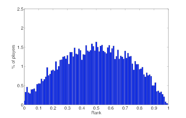
A subject’s local rank is the proportion of subjects who answered a particular question faster than he did. It is calculated for each participant for each of the questions he answered. A global rank is calculated for each subject who answered at least 9 problems. The median number of answers for a subject who received a global rank is 15. About 50% of the subjects received global rank. A subject’s global rank is the median of his local rankings. Figure 1 presents the frequency distribution of global rankings.
Figure 1: The frequency distribution of global rankings.
Note that an individual’s local ranking is by definition sampled from a uniform distribution in the interval [0,1]. If the local ranks of the same individual were sampled independently, we would obtain a distribution that is close to normal with a mean of 0.5 and a standard deviation of less than 0.1. However, the distribution of global rankings in Figure 1 is far more dispersed (in particular, notice that only 29% lie within one standard deviation from 0.5 and only 55% within two standard deviations). Therefore, it appears that the classification of a subject as high or low in the global rankings is not just a matter of statistical coincidence.
The correlation between the respondents’ local and global ranks was calculated for each problem. With one exception, it always lies within the interval (0.5, 0.7) and is usually in the vicinity of 0.6.
For each problem, n and m were calculated as follows:
n - the total number of subjects who responded to the question.
m - the total number of subjects who responded to the question and also have a global rank.
Data will be presented in three forms:
a. Graphs: A graph will include the basic statistics of the distribution of answers and the corresponding MRT and will present the cumulative distributions of the main responses.
b. Tables: A table will present the distribution of answers and their MRT for subjects responding to a particular problem, according to their local and global ranking quartiles.
In cases where subjects responded to two related problems, two tables will be presented: one “local” and the other “global”. Each table presents two joint distributions: one for the “fast” responders and one for the “slow” responders. In a “local” table, the slow (fast) responders are those who responded slower (faster) than the median in both problems. Typically, about 75% of the subjects are included in these two equally-sized groups. In the “global” tables, the slow (fast) responders are those with global ranking above (below) the median global ranking (in this case, the two groups are only approximately of equal size).
This section presents four problems in which the response time results are consistent with the hypothesis that response is significantly faster for choices that clearly involve a mistake.
The “Count the Fs” problem has been circulating on the Internet for a number of years. (I don’t know its origin.) Subjects were asked to count the number of appearances of the letter F in the following 80-letter text:
yellowFINISHED FILES ARE THE RE- yellowSULT OF YEARS OF SCIENTIF- yellowIC STUDY COMBINED WITH yellowTHE EXPERIENCE OF YEARS.
Defining a mistake is straightforward in this case: either the number of F’s is counted correctly or not. Many readers will be surprised to learn that the right answer is 6 and not 3. In fact, only 37% of the subjects (n=5324 and m=4453) answered the question correctly. The reason is that many people (including myself) tend to skip the word “of” when reading a text and in the above text it appears three times. Only 3% of the subjects gave an answer outside the range 3-6. This can be taken as evidence that subjects took the task more seriously than some critics would claim. The graphs in Figure 2 present a clear picture in this case.
Figure 2: Count the Fs: Basic results for the answers 3,4,5 and 6 (about 3% of subjects gave a different answer) 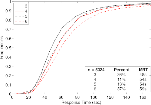
Subjects who made a large mistake (i.e. they answered 3) spent about 6s less on the problem than those who answered “4” or “5” and 11s less than those who answered “6”. Note the similarity in response times between the answers “4” and “5”. In some sense, “4” is a “bigger” mistake than “5”. However, note that the word “of” appears twice in the second line and once in the last line. It seems reasonable to assume that a person who notices one of the ”of” ’s in the second line will also notice the other. Thus, the ”size” of the mistake is in fact similar for the subjects who chose “4” or “5”.
Table 1: Count the Fs: Results according to local and global rankings for the answers 3,4,5 and 6 (about 3% of subjects gave a different answer)
Local ranking quartiles Global ranking quartiles Response Fastest Fast Slow Slowest Fastest Fast Slow Slowest 3 46% 42% 31% 26% 43% 36% 34% 29% 4 11% 11% 12% 11% 12% 12% 10% 10% 5 13% 13% 14% 12% 13% 12% 14% 13% 6 29% 32% 41% 46% 29% 37% 39% 45% n 1331 1331 1331 1331 1134 1166 1145 1008 MRT 31s 46s 62s 98s 39s 50s 59s 80s
Table 1 presents the distribution of the answers 3, 4, 5 and 6 in each of the four quartiles (the few answers below 3 and above 6 are not reported). According to the local rankings, the proportion of “large” mistakes among the slowest quartile of subjects is 26% whereas it is 46% among the fastest. Furthermore, 46% of the slowest participants gave the correct answer as compared to only 29% of the fastest. Similar though less pronounced differences were obtained for global rankings.
Figure 3: Most likely sequence: Basic results 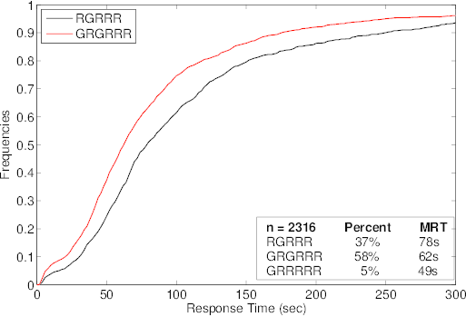
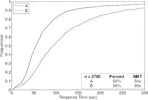
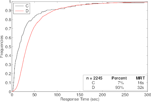
Figure 4: The two roulette games: Basic results
Kahneman and Tversky (1983) report on the following experiment:
Subjects were asked to consider a six-sided die with four green faces and two red ones. The subjects were told that the die will be rolled 20 times and the sequence of G and R recorded. Each subject was then asked to select one of the following three sequences and told that he would receive $25 if it appears during the rolls of the die. The three sequences were:RGRRR
GRGRRR
GRRRRR
The right answer is of course RGRRR (results are presented in Figure 3). Only 5% of the subjects (n=2316 and m=2159) chose the blatantly incorrect answer GRRRRR, although 58% chose the other mistake GRGRRR (note that whenever this sequence appears, RGRRR appears as well). The MRT for the right answer is much higher (by 16s) than for the mistake, which is the far more common answer.
Table 2: Most likely sequence: Results according to local and global rankings.
Local ranking quartiles Global ranking quartiles Response Fastest Fast Slow Slowest Fastest Fast Slow Slowest RGRRR 26% 34% 40% 47% 28% 36% 42% 43% GRGRRR 66% 62% 57% 49% 66% 59% 54% 53% GRRRRR 8% 5% 3% 4% 6% 5% 4% 4% n 579 579 579 579 544 560 550 505 MRT 26s 54s 85s 173s 34s 59s 80s 136s
According to the local rankings (see Table 2), 47% of the slowest quartile of subjects gave the correct answer as compared to only 26% of the fastest quartile. Similar differences were obtained for the global rankings. The correlation between the local and global rankings is 0.64.
Tversky and Kahneman (1986) demonstrated the existence of framing effects using the following experiment. Subjects are asked to (virtually) choose between two roulette games:
| White | Red | Green | Yellow | ||
| Game A: | Chances % | 90 | 6 | 1 | 3 |
| Prize $ | 0 | 45 | 30 | −15 | |
| Game B: | Chances % | 90 | 7 | 1 | 2 |
| Prize $ | 0 | 45 | −10 | −15 |
Subjects were divided almost equally between choosing A and B (n=2785, m=2319). The choice of A is probably an outcome of using a “cancelling out” procedure in which similar parameters (Red and Yellow) are ignored and subjects focus on the large differences in the Green parameter ($30 vs -$10). However, choosing according to Green is a mistake since A and B are “identical” to C and D respectively (n=2245, m=1854) and D clearly “dominates” C:
| White | Red | Green | Blue | Yellow | ||
| Game C: | Chances % | 90 | 6 | 1 | 1 | 2 |
| Prize $ | 0 | 45 | 30 | −15 | −15 | |
| Game D: | Chances % | 90 | 6 | 1 | 1 | 2 |
| Prize $ | 0 | 45 | 45 | −10 | −15 |
Table 3: The two roulette games: Results according to local and global rankings.
Local ranking quartiles Global ranking quartiles Response Fastest Fast Slow Slowest Fastest Fast Slow Slowest A 70% 59% 44% 25% 61% 56% 48% 36% B 30% 41% 56% 75% 39% 44% 52% 64% n 696 696 696 697 525 570 632 592 MRT 30s 56s 89s 185s 35s 59s 82s 142s
The RT results, presented in Figure 4, dramatically confirm that making a wrong choice is correlated with shorter RT.
Among subjects in the local ranking fastest quartile (see Table 3), 70% chose A and 30% chose B while among the slowest quartile, 25% chose A and 75% chose B. The global ranking is a strong predictor of response time in this problem. While 61% of the fastest responders chose A, 64% of the slowest responders chose B.
Another interesting example is the Wason (1960) experiment:
Suppose that there are four cards in front of you, each with a number on one side and a letter on the other. The cards before you show the following:4 U 3 MWhich cards should you turn over in order to determine the truth of the following proposition: If a card has a vowel on one side, then it has an even number on the other?
The right answer, i.e. U and 3, was selected by only 10% of the subjects (n=2000, m=1773). The three most commonly made mistakes are 4 and U (21%), all (23%) and U (13%). Once again, the results (see Figure 5 and Table 4) reveal a strong correlation between choosing the right answer and high response time.
Table 4: The Wason experiment: Results according to local and global rankings.
Local ranking quartiles Global ranking quartiles Response Fastest Fast Slow Slowest Fastest Fast Slow Slowest U 15% 15% 12% 10% 13% 14% 11% 10% 4+U 17% 26% 21% 20% 20% 22% 22% 19% U+3 6% 8% 12% 14% 7% 11% 10% 12% All 20% 24% 23% 24% 18% 22% 29% 28% n 500 500 500 500 480 466 420 407 MRT 38s 71s 116s 245s 47s 78s 114s 190s
Figure 5: The Wason experiment: Basic results 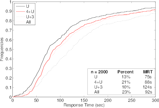
The low proportion of subjects who made the correct choice makes it difficult to draw any further conclusions. What can be said is that, according to the local ranking results, 14% of the slowest quartile (MRT of 250 seconds) responded correctly, in contrast to only 6% of the fastest quartile (MRT of 31 seconds). Similarly, there is a significant difference in the proportions of correct answers between the two extreme quartiles of responders as partitioned by the global ranking.
The previous section presented four distinct problems, in which the notion of a mistake was well defined, in order to demonstrate the correlation between short response time and mistakes. This section presents the results of an experiment in which the correlation between mistakes and response time appears to be reversed and offers an explanation of the result.
Most of the 729 subjects were PhD or MA level students in microeconomics courses in at Tel Aviv University and New York University who responded to a questionnaire consisting of 36 questions about nine vacation packages. In each of the questions, the subject was asked to compare two packages (with three possible responses: 1. I prefer the first alternative; X. I am indifferent between the alternatives; and 2. I prefer the second alternative). Each vacation package was described in terms of four parameters: destination, price, level of accommodation and quality of the food. The destination (either Paris or Rome) was always presented first, followed by the other three parameters in arbitrary order.
The goal of this rather tedious questionnaire was to demonstrate the concept of preferences and to show the students that even they (i.e. economics students) often respond in a way that violates transitivity as soon as the alternatives become even slightly complicated.
What constitutes a mistake in this case is clear. People are known to be embarrassed when they discover that their answers are not transitive (i.e. for some three alternatives x ≻ y and y ≻ z but not x ≻ z, or x ∼ y and y ∼ z but not x ∼ z). A cycle is a three-element set {x, y, z} when one of these two configurations appears in a subject’s answers.
Figure 6 presents the distribution of number of cycles. Only 12% of the subjects did not exhibit a violation of transitivity. The median number of cycles was 7 and the number of cycles varied widely—from 0 to 58!5 Thus, even PhD students in economics often violate transitivity.
Figure 6: The distribution of cycles 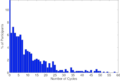
Note that two of the alternatives were actually identical:
“A weekend in Paris at a 4-star hotel with a Zagat food rating of 17 for $574” and
“A weekend in Paris for $574 with a Zagat food rating of 17 at a 4-star hotel”.
Almost all the subjects (91%) expressed indifference between the two alternatives. However, the three most common cycles (each of which appears in the responses of 22–29% of the subjects) involve those alternatives.
We now return to response time. Figure 7 presents the cumulative response time distributions for subjects whose number of mistakes is “between 0 and 3” and “above 3” (similar graphs are obtained for other nearby cutoff points).
Figure 7: The preference questionnaire: RT distributions. 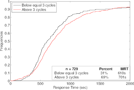
Table 5: The preference questionnaire: Local rankings.
Local ranking quartiles Number of “cycles” Fastest Fast Slow Slowest 3 and below 38% 32% 31% 24% 4 and above 62% 68% 69% 76% n 182 183 182 182 MRT 387s 563s 813s 1398s
In contrast to Section 2, here we find that shorter response time is correlated with fewer mistakes. The MRT of those subjects with a small number of cycles is 90 seconds (!) less than the MRT of the others. Table 5 presents the results by quartiles of the local rankings.6
A plausible explanation of the “anomaly” is that consistent answers might be an outcome of activating a simple rule which does not require a long response time (such as “I prefer one alternative over another based only on comparing their prices”). Looking more closely at the responses of the subjects whose answers are consistent with transitivity provides support for this intuition. Of the 84 “transitive responses”, 4 exhibited simple constant indifference and for another 48 responses one can identify a dimension that was the subject’s lexicographic first priority (location (29), price (12), level of accommodation (4) and quality of the food (3)). Correctly applying a more complicated rule that produces no intransitivities is more likely to lead to mistakes. Thus, consistency with transitivity may reflect the use of a simple rule rather than greater sophistication (this conclusion conflicts with Choi, Kariv, Müller and Silverman (2011)’s approach).
In this section, we discuss the results of three problems that are often used in the literature to demonstrate the high incidence of behavior that conflicts with established theories. Each problem consists of a pair of questions. The standard theories predict a one-to-one correspondence between the answers to the two questions. The standard experimental protocol requires that subjects be randomly divided between the two problems, which makes it possible to treat the two populations as identical. If the proportion of those who chose a particular alternative in one question differs from that in the other question, this is interpreted as being inconsistent with the theory. A different protocol is used here. In each of the examples, subjects were asked to answer the two questions sequentially in the order they are presented here. The results are robust to this change in the protocol and inconsistent behavior remains very common, even though subjects could have easily detected the inconsistency.
The following is Kahneman and Tversky (1979)’s well-known version of the Allais paradox:
A1: You are to choose between the following two lotteries:
Lottery A which yields $4000 with probability 0.2 (and $0 otherwise).
Lottery B which yields $3000 with probability 0.25 (and $0 otherwise).
Which lottery would you choose?
A2: You are to choose between the following two lotteries:
Lottery C which yields $4000 with probability 0.8 (and $0 otherwise).
Lottery D which yields $ 3000 with probability 1.
Which lottery would you choose?
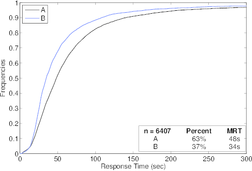
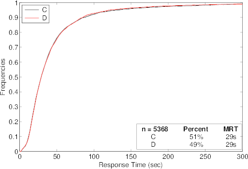
For completeness, Figure 8 presents the basic results (n=6407, m=5195 for A1 and n=5639, m=4588 for A2).
Figure 8: Allais Paradox: Basic results
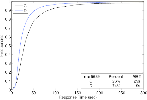
Note that the choice of the less risky options (B and D) is associated with much shorter RT than the corresponding options (A and C, respectively). The fact that response time is faster in problem A2 than in A1 is due to two factors: First, A2 was presented after A1 and therefore subjects were already familiar with this type of question. Second, based on the responses of those who answered only one of the two questions, it can be inferred that A2 is simpler than A1.
However, my main interest in analyzing these results lies elsewhere. Recall that the Independence axiom requires that the choices of a decision maker in each of the two problems be perfectly correlated. In other words, we should observe two types of decision makers: those who are less risk averse and choose A and C and those who are more risk averse and choose B and D. The standard typology of agents in economics is based on their attitude towards risk (often captured by the estimated coefficient of a Constant Elasticity of Substitution utility function).
Table 6: Allais Paradox: Joint distribution of the responses. The numbers in parentheses indicate the expected joint distribution if the answers to the two questions were independent.
n = 5528 C D Total A 20% (16%) 44% (47%) 64% B 5% (9%) 31% (27%) 36% Total 25% 75% 100%
There are 5528 subjects who responded to both problems, one after the other. Table 6 presents the joint distribution of their responses. Note that 49% of the subjects exhibited behavior that is inconsistent with the Independence axiom. The hypothesis that the answers to the two problems are independent is rejected; however, the experimental joint distribution is not that far from the distribution expected if the answers to the two problems were totally independent (this distribution appears in parentheses). This finding (unrelated to RT) casts doubt on the basic typology that is commonly used to classify behavior under uncertainty. Would another typology perhaps explain the results better?
We now turn to the data on response time. A point in Figure 9 represents a single subject. The coordinates (x, y) represent the pair of his local rankings (the proportion x of the population responded faster than he did to A1 and the proportion y responded faster than he did to A2).
Figure 9: Allais Paradox: Local rankings for A1 and A2. 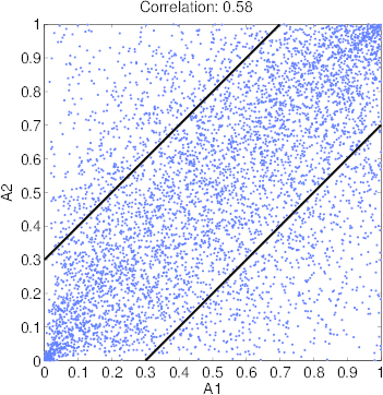
The correlation between the two relative positions is 0.58. Note that the vast majority of subjects fall within the area (of size ½) between the two diagonal lines. The high correlation suggests that there is a meaning to examine the behavior of subjects who were consistently fast or slow in responding to this particular pair of problems.
Table 7: Allais Paradox: Joint distribution according to local ranking and according to global ranking. In the “local” table, the slow (fast) responders are those who responded slower (faster) than the median in both problems. In the “global” table, the slow (fast) responders are those with global ranking above (below) the median. In each table, fast subjects appear in the upper left-hand corner of the cell and slow subjects in the bottom right-hand corner.
According to Local Ranking Fast C D Total Slow A 12% 43% 55% 33% 42% 75% B 5% 40% 45% 5% 20% 25% Total 17% 83% n = 1983 37% 63% n = 1983 According to Global Ranking Fast C D Total Slow A 17% 44% 62% 25% 43% 68% B 5% 33% 38% 5% 27% 32% Total 22% 78% n = 2373 30% 70% n = 2129
Table 7 presents the joint distributions of responses according to local and global rankings. There are two striking patterns in the results: First, the choices of the slow group were no more consistent with the Independence axiom than those of the fast group. Thus, longer response time appears to contribute little to consistency. The choices of 52% of the fast subjects and 53% of the slow subjects were consistent with the Independence axiom. This result supports the view that the inconsistency of the choices with expected utility theory is not simply an outcome of error.
Second, the pattern of those choices that are consistent with expected utility theory differs dramatically between the groups. While almost 4/5 of the fastest consistent subjects chose B and D, less than 2/5 of the slowest consistent subjects chose that combination.
These results suggest that theoretical models should be based on a two-element typology (see Rubinstein, 2008). This will involve a Fast type who either behaves intuitively (i.e., chooses A and D) or exhibits risk aversion (i.e. chooses B and D) with equal probability. A Slow type will either behave intuitively (i.e., choose A and D) or maximize expected payoff (i.e., choose A and C) with equal probability. Further research is needed in order to provide a stronger footing for such a typology.
The Ellsberg Paradox was presented to students in the following two versions (almost all students answered E1 first):
E1. Imagine an urn known to contain 30 red balls and 60 black and yellow balls (in an unknown proportion). One ball is to be drawn at random from the urn. The following actions are available to you: “bet on red”: yielding $100 if the drawn ball is red and $0 otherwise. “bet on black”: yielding $100 if the drawn ball is black and $0 otherwise. Which action would you choose?
E2. Imagine an urn known to contain 30 red balls and 60 black and yellow balls (in an unknown proportion). One ball is to be drawn at random from the urn. The following actions are available to you: “bet on red or yellow”: yielding $100 if the drawn ball is red or yellow and $0 otherwise. “bet on black or yellow”: yielding $100 if the drawn ball is black or yellow and $0 otherwise. Which action would you choose?
Table 8: Ellsberg: Joint distribution of the responses. The numbers in parentheses indicate the expected joint distribution if the answers to the two questions were independent (n = 1791).
E2 Red or yellow Black or yellow Total E1 Red 15% (13%) 49% (51%) 64% Black 6% (7%) 30% (28%) 36% Total 21% 79% 100%
The results do not show any significant correlation between the responses to the two questions. Table 8 presents the joint distribution of the responses.
However, my main interest lies in whether the “inconsistent” choice, mainly “red” in E1 and “black or yellow” in E2, is correlated with short response time. Table 9 is structured like Table 7.
Table 9: Ellsberg Paradox: Joint distribution according to local ranking and according to global ranking.
According to Local Ranking Fast Red or Black or Total Slow yellow yellow Red 19% 46% 66% 11% 50% 61% Black 7% 28% 34% 6% 33% 39% Total 26% 74% n = 625 17% 83% n = 626 According to Global Ranking Fast Red or Black or Total Slow yellow yellow Red 18% 47% 65% 11% 52% 63% black 6% 29% 35% 6% 31% 37% Total 24% 76% n = 771 18% 82% n = 826
The proportion of consistent subjects is actually slightly higher among the fast responders according to both the local and global rankings (for example, according to the local ranking 47% of the fast responders and 44% of slow responders were consistent). Among the consistent subjects, there is a difference in behavior between the fast and slow groups, although it is less dramatic than in the Allais Paradox.
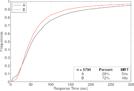
Kahneman and Tversky (1986) proposed the famous “outbreak of disease” experiment:
KT1. The outbreak of a particular disease will cause 600 deaths in the US. Two mutually exclusive prevention programs will yield the following results: A: 400 people will die. B: With probability 1/3, 0 people will die and with probability 2/3, 600 people will die. You are in charge of choosing between the two programs. Which would you choose?
KT2. The outbreak of a particular disease will cause 600 deaths in the US. Two mutually exclusive prevention programs will yield the following results: C: 200 people will be saved D: With probability 1/3, all 600 will be saved and with probability 2/3 none will be saved. You are in charge of choosing between the two programs. Which would you choose?
Figure 10: Outbreak of Disease: Basic statistics
The results (see Figure 10) are similar to those of Kahneman and Tversky. KT1 was presented first and 28% of the subjects (vs. 22% in the original experiment) chose A (n=5694, m=5221). B appears to be the more instinctive choice in this case (especially if we ignore the very fast-responding tail of the distribution). Remarkably, the two RT distributions for those who chose C or D in KT2 are almost identical. The fact that 49% of the subjects (vs. 28% in the original experiment) chose D in KT2 is partially a result of KT2 being presented to the same subjects subsequent to KT1 (Kahneman and Tversky followed the standard protocol and gave the two questions to two different populations). Note, however, that 44% of a small sample of 91 subjects who answered only KT2 chose D.
Table 10: Outbreak of Disease: Joint distribution of the responses (n = 5277).
C D Total A 23% (14%) 5% (14%) 28% B 28% (36%) 44% (35%) 72% Total 51% 49% 100%
A large proportion of subjects (67%) exhibited consistent behavior in this problem (see Table 10), whereas only 49% would be expected to do so if the choices were independent.
The distributions of the Fast and Slow subjects, as classified by the local or global ranking, are remarkably similar (see Table 11). This tends to indicate that a meaningful typology of subjects in this context should not in fact be based on the Fast/Slow categories.
Table 11: Outbreak of Disease: Joint distribution according to local ranking and according to global ranking.
According to Local Ranking Fast C D Total Slow A 22% 7% 29% 24% 5% 29% B 27% 44% 71% 28% 44% 71% Total 49% 51% n = 1837 52% 48% n = 1838 According to Global Ranking Fast C D Total Slow A 21% 6% 27% 24% 5% 28% B 29% 44% 73% 27% 45% 72% Total 50% 50% n = 2412 51% 49% n = 2409
The line of argument presented above can be summarized as follows:
a) Section 2 presented four problems (counting the F’s, comparing the likelihood of two sequences, choosing between roulettes and the Wason Experiment) in order to demonstrate that when the notion of a mistake is a clear cut there is a strong correlation between short response time and mistakes.
b) Section 3 showed that an inverse relation between short response time and making a mistake may appear in certain situations (such as when making 36 comparisons between pairs of alternative) due to the use of a simple choice rule that may be associated with making less mistakes.
c) Section 4 showed that short response time is not associated with behavior that conflicts with the standard theories, which are typically violated by Allais, Ellsberg and Kahneman-Tversky framing paradoxes. Behavior that is not consistent with Expected Utility Theory and is sensitive to framing effects appears among fast and slow responders in similar frequencies.
d) I began this research with the goal of finding strong correlations in the choice behavior of subjects in different contexts. I was able to detect strong correlations between the relative speed of subjects responding to several problems. In some cases (especially that of the Allais paradox), the results suggest that classifying subjects as fast or slow responders is useful. Additional research is needed to establish this point.
However, I was unable to detect more than a weak correlation in behavior across choice problems, unless the problems were similar to one other. There are those who will be disappointed by this result. I however feel that the difficulty in predicting a person’s behavior (based on his past behavior) is a positive result, which affirms an individual’s freedom of action, in a sense.
Whatever reservations one might have regarding the method and analysis, I hope that it has at least suggested that response time is an interesting tool in the evaluation of experimental results.
Agranov, M., Caplin, A., & Tergiman, C. (2012). Naïve play and the process of choice in guessing games. New York Univeristy, Working Paper.
Arad, A., & Rubinstein, A. (2012). Multi-Dimensional Iterative Reasoning in Action: The Case of the Colonel Blotto Game. Journal of Economic Behavior & Organization, 84, 571–585.
Brañas-Garza, P., Meloso, D., & L. Miller. (2012). Interactive and moral reasoning: A comparative study of response times. Innocenzo Gasparini Institute for Economic Research, Bocconi University, Working Paper 440.
Choi, S., Kariv, S., Müller, W., & Silverman, D. (2011). Who is (more) Rational?. National Bureau of Economic Research, Working Paper 16791.
Chabris, C.F., Laibson, D., Morris, C.L., Schuldt, J.P., & Taubinsky, D. (2009). The allocation of time in decision-making. Journal of the European Economic Association, 7, 628–637.
Donders, F.C. (1969). On the speed of mental processes. Acta psychologica, 30, 412–431.
Gigerenzer, G., Krauss, S. , & Vitouch, O. (2004). The null ritual: What you always wanted to know about significance testing but were afraid to ask. In: D. Kaplan (Ed.). The Sage handbook of quantitative methodology for the social sciences, pp. 391–408. Thousand Oaks: Sage.
Hertwig, R., Fischbacher, U., & Bruhin, A. (2013). Simple heuristics in a social game. In R. Hertwig, U. Hoffrage, & the ABC Research Group, Simple heuristics in a social world, pp. 39–65. New York: Oxford University Press.
Kahneman, D. (2011). Thinking, Fast and Slow. New York: Farrar, Straus and Giroux.
Kahneman, D., & Tversky, A. (1979). Prospect Theory: An Analysis of Decision Under Risk. Econometrica, 47, 263–292.
Lotito, G., Migheli, M., & Ortona, G. (2011). Is cooperation instinctive? Evidence from the response times in a public goods game. Journal of Bioeconomics, 13, 1–11.
Piovesan, M. & Wengström, E. (2009). Fast or fair? A study of response times. Economics Letters, 105, 193–196.
Read, D. (2005). Monetary incentives, what are they good for? Journal of Economic Methodology, 12, 265–276.
Rubinstein, A. (2001). A Theorist’s View of Experiments. European Economic Review, 45, 615–628.
Rubinstein, A. (2007). Instinctive and Cognitive Reasoning: A Study of Response Times. The Economic Journal, 117, 1243–1259.
Rubinstein, A. (2008). Comments on NeuroEconomics. Economics and Philosophy, 24, 485–494.
Schotter, A., & Trevino, I. (2012). Is response time predictive of choice? An experimental study of threshold strategies. A discussion paper, New York University.
Sternberg, S. (1969). Memory-scanning: Mental processes revealed by reaction-time experiments. American Scientist, 57, 421–457.
Tversky, A., & Kahneman, D. (1983). Extensional versus intuitive reasoning: The conjunction fallacy in probability judgment. Psychological Review, 90, 293–315.
Tversky, A., & Kahneman, D. (1986). Rational Choice and the Framing of Decisions. The Journal of Business, 59, 251–278.
Wason, P. C. (1968). Reasoning about a rule. The Quarterly Journal of Experimental Psychology, 20, 273–281.
Copyright: © 2013. The author licenses this article under the terms of the Creative Commons Attribution 3.0 License.
This document was translated from LATEX by HEVEA.