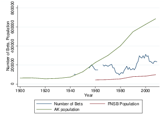
| Figure 1: Population of Alaska and the Fairbanks North Star Borough and NIC bets since 1900, for years where data are available. |
Judgment and Decision Making, vol. 8, no. 2, 2013 2013, pp. 91-105
The wisdom of crowds: Predicting a weather and climate-related eventKarsten Hueffer* Miguel A. Fonseca# Anthony Leiserowitz% Karen M. Taylor% |
Environmental uncertainty is at the core of much of human activity, ranging from daily decisions by individuals to long-term policy planning by governments. Yet, there is little quantitative evidence on the ability of non-expert individuals or populations to forecast climate-related events. Here we report on data from a 90-year old prediction game on a climate related event in Alaska: the Nenana Ice Classic (NIC). Participants in this contest guess to the nearest minute when the ice covering the Tanana River will break, signaling the start of spring. Previous research indicates a strong correlation between the ice breakup dates and regional weather conditions. We study betting decisions between 1955 and 2009. We find the betting distribution closely predicts the outcome of the contest. We also find a significant correlation between regional temperatures as well as past ice breakups and betting behavior, suggesting that participants incorporate both climate and historical information into their decision-making.
Keywords: decision-making under uncertainty, wisdom of
crowds, natural experiment, environmental decision-making.
The Wisdom of Crowds effect (WoC) is the empirical observation that groups tend to make more accurate predictions than individuals, even when some individuals may have a particular expertise in the phenomenon being predicted. An early example of the WoC goes back to the 1920s, where social psychology students were asked to individually estimate air temperature in a classroom. (See Larrick & Soll, 2006 for a historical review.) The average of the individual guesses turned out to be more accurate than most individuals’ guesses.
The fundamental basis to the WoC phenomenon lies in the way a group’s prediction aggregates different types of information or opinions from its constituents. At a primary level, the simple fact that the prediction of a large group of individuals is an aggregation of opinions (e.g., the average opinion) will by construction rule out extreme errors (Clemen, 1989). However, this principle does not ultimately guarantee that the group’s forecast is a good predictor, or that it is any better than the prediction made by an expert.
The literature on the WoC instead argues that groups can be more accurate than most individuals to the extent to which each group is diverse. This diversity may lie in differences in individual skill sets of group members, or different members may have access to different sources of information (Surowiecki, 2004; Soll, Mannes, & Larrick, 2011). This possibility of aggregating diverse information makes groups more effective than individuals at making predictions, in a similar manner to prediction markets but, importantly, without a market price as a coordination mechanism.
Larrick, Mannes & Soll (2012) review the literature on the WoC, and discuss the conditions under which crowds are wise. They identify expertise and diversity as necessary properties that enable groups to be effective forecasters. Crowds must have expertise in the sense that they are making judgments about something they know or have experienced—the problem should not be new. The authors argue that diversity has as much to do with the composition of the group (and the different individual forecasts that will be then aggregated), as with the way individual forecasts are aggregated.
While the need for diversity in the composition of the group is intuitive, the need for particular mechanisms through which individuals interact and information and/or decisions are aggregated deserves closer attention. In the absence of prices as a coordination device, group members may base their own judgments on social cues (what Tversky & Kahneman, 1974 termed “anchoring”). Furthermore, if the mechanism through which the group aggregates decisions is sequential and the decisions are public, there is a potential for information cascades to form. That is, members may disregard their own private information when making their prediction if they observe sufficiently many group members predicting the same outcome. (See Anderson & Holt, 1997 for early experimental evidence on informational cascades; and see Bikhchandani, Hirschleifer, & Welch, 1998 for a review.) This possibility has led some (Armstrong, 2006) to argue, perhaps paradoxically, that group forecasts maybe best made if individual predictions are made without any contact between group members.
In the present paper, we test the Wisdom of Crowds hypothesis using data from a climate-related betting game. In particular, we test the ability of a betting game to accurately forecast a highly variable natural event (ice breakup dates) in the midst of a distinct climate shift over the course of several decades. We draw upon a unique data set from a longstanding natural experiment, the Nenana Ice Classic, to examine perceptions of a climate-related event over the last century. Each year since 1917, participants from across Alaska place bets on the exact date and time when the ice covering the Tanana River will break up, signaling the start of spring. The closest bet to the nearest minute wins a prize of up to $300,000. The Nenana Ice Classic forms an integral part of the social calendar in Alaska, receiving significant coverage from the local press (Arctic Science Journeys, 1997; Finkel, 1998).
Figure 1: Population of Alaska and the Fairbanks North Star Borough and NIC bets since 1900, for years where data are available.
The object of this prediction game is also interesting in itself. The Arctic has experienced increases in average winter temperature twice as large as the rest of the world (Bord, Fisher, & O’Connor, 1998). Therefore, this region is ideal for the study of changes in local and regional perceptions of climate-related events. The historical breakup record of the Tanana River over the course of the 20th century demonstrates a long-term trend towards earlier breakup (i.e., an earlier onset of spring), in line with earlier work indicating the ice melt in Nenana follows instrumental records indicating a warming trend throughout the Arctic from 1970 to 2001 (Sagarin & Micheli, 2001).
The longstanding record of this betting pool makes the historical record of the ice breakup a useful source of data to study climate events. Sagarin & Micheli (2001) found a correlation between warmer winter months and earlier breakups, based on regional air temperature records. From the perspective of the participants of the betting pool, apart from the historical record of break-up dates, weather data is one of the most likely sources of information used to make betting decisions: a colder winter is likely to lead to a later break-up of the ice. This conjecture is corroborated by reports from the popular press, as well as from the organizers of the NIC, of general interest in weather conditions around the time when betting takes place (Richards, 1995; Arctic Science Journeys, 1997). This interest is reflected in close coverage of weather conditions by local media during the time when bets are allowed (Finkel, 1998).
Insofar as we are interested in studying the information upon which individuals make their forecasting decisions, the mechanism in this natural experiment also has an advantage relative to “standard” prediction markets.1 In standard prediction markets like the Iowa Electronic Markets,2 buyers and sellers continuously post buy and sell orders while observing current prices. These prices convey the contemporaneous information about the likelihood of a given event occurring—typically shares pay out $1 in case of a correct prediction and $0 otherwise, which leads one to interpret the price as a probability. As such, when a trader makes a trading decision in a market, it is very difficult to establish the extent to which the trader is relying on the public information conveyed by the price, or his/her private information.
The Nenana Ice Classic participants must place their bets between February and April of each year, which is typically one to two months before the ice breaks. The large number of bettors, spread across Alaska, and the fact that the actual record of bets is only publicized after the ice breaks up means that each individual is likely to rely only on her private information when making her betting decision.3
The NIC betting pool is a “wise crowd” while not being a prediction market in the standard sense: prediction markets use prices to coordinate and update beliefs about some event happening, while wise crowds are diverse groups of individuals who share expertise on that event (Larrick, Mannes and Soll, 2012). As such, even a simple betting pool could meet the conditions for a wise crowd. The NIC crowd meets the criteria for a wise crowd. It forecasts a very well-defined event. The crowd’s expertise comes from local experience of weather and climate conditions, as well as historical knowledge of past break-ups. The NIC crowd is particularly experienced in that regard, as the contest has been in existence for the best part of a century.
Furthermore, the set of NIC participants is a very large and diverse group of individuals. Bettors are spread across Alaska, and as such they will have access to a wide variety of information sources and skill sets, as we will argue below. Moreover, individual participants place their bets independently without any knowledge of what the overwhelming majority of the group has done. This essentially eliminates the role of information cascades and conformity. Finally, participants are playing for very high stakes, making the incentives to get a correct answer quite salient.
All in all, this natural experiment gives us a unique insight into the ability of a population to predict a well defined and naturally occurring event, and to understand the mechanisms behind the aggregation of information in large groups.
We find that the aggregated prediction by Nenana Ice Classic participants is a reasonably good predictor of the actual ice break-up date. It does not underperform a set of models based on contemporaneous weather information. It slightly outperforms models solely based on past break-up information. This result hints at the fact that NIC participants may use contemporaneous weather information in addition to historical break-up data to inform their decisions. An econometric analysis of the time series of predictions lends support to this hypothesis. The following section provides some background on the natural experiment we analyze. Section 3 describes the data and Section 4 reports on the results. Section 5 concludes the paper.
The city of Nenana in central Alaska is the home of one of the oldest annual prediction games in the world. In 1917, a group of surveyors decided to form a betting pool to predict when the ice covering the nearby Tanana River would break, signalling the start of spring. Popular interest in the lottery increased over the years and the Nenana Ice Classic now receives over 200,000 bets every year, handing out over $300,000 in prize money (Figure 1).
The rules of the betting pool are simple: every year a tripod is set up on top of the ice covering the Tanana River. This tripod is connected to a clock on the riverbank recording the date and time. When the ice surface collapses during the spring, the device automatically records the date and time (to the nearest minute) when the tripod fell into the water.4 As such, each individual placing a bet must indicate the exact date and time when the tripod will fall. Whoever is closest to the actual time wins the whole pot; in the event of a tie, the prize is divided equally among the winners.
The WoC predicts that behavior by the set of participants in the Ice Classic will be more accurate than any expert. Before we compare the performance of the crowd to that of experts, it is reasonable to ask if the crowd’s prediction is accurate at all. If the crowd is at all wise, its predictions should be accurate. This constitutes our first hypothesis:
The median of the distribution of bets in the Nenana Ice Classic will be an accurate predictor of the timing of the ice break-up.
An important assumption in the WoC is that the population, whether through private information, observation of the environmental conditions as well as the past outcomes of the NIC, uses all available sources of information to produce its forecast. As such, we would expect the current climate conditions to be correlated with betting behavior. This leads us to the next hypothesis:
Climate conditions at the time of betting will correlate with the prediction of the betting population.
If indeed the prediction of the betting pool is accurate and based on reasonable sources of information, we can then postulate the main hypothesis of the paper:
The prediction made by the betting pool will be more accurate than that of any “expert”, which we define as an omniscient statistical model of the break-up date using relevant information, such as climate information and/or past break-up dates.
An alternative to the hypothesis that the crowd will effectively use weather and historical data is that, because they are boundedly-rational, bettors will resort to rules of thumb when making their decisions. The representativeness heuristic (Tversky & Kahneman, 1974) is particularly appropriate to our data set. It states that individuals will make judgments about the likelihood of a particular event while ignoring the base-rate frequency of events. That is, individuals make inferences about a distribution of outcomes based on a small subset of (typically recent) draws from that distribution.
Evidence from laboratory experiments (Grether, 1992) suggests that individuals rely upon the representativeness heuristic when making repeated decisions under uncertainty. There is also field evidence to support this conjecture: Jorgenson, Suetens & Tyran (2011) and Suetens & Tyran (2012) look at betting data from the Danish lottery and find that Danish bettors are prone to the “hot hand fallacy”—picking lotto numbers which have been drawn in consecutive weeks, a phenomenon consistent with representativeness. See Oskarsson et al. (2009) for a comprehensive survey on this literature, as well as a theoretical framework for mental models of decision-makers’ beliefs on binary events.
In our framework, this means that participants of the NIC will overweight break-up dates in the recent past when constructing their probability estimates for the year in which they are betting.
Subjects’ betting decisions will be disproportionally influenced by break-up dates in the recent past.
NIC tickets are sold throughout Alaska between February 1st and April 5th each year. Only one bet is allowed per ticket, and each ticket costs $ 2.50. The prize money is a function of the total revenue from betting. Historical data on past break-up dates and times are tabulated in calendar form on the brochure that accompanies the NIC betting form. The presentation of these data, however, does not provide an intuitive visual description such as a histogram, and requires significant further analysis from participants in order to extract more sophisticated information, such as time trends.
Participants must provide their name, address and predicted break-up date and time. The NIC team then compiles the betting records into the NIC Book of Guesses. The format of the book has remained consistent over the decades. Since it is impractical to scan each Book of Guesses and digitize all the data, we took advantage of the fact that each book has a fixed number of entries per page, which are ordered by the predicted date and time of break-up. Given the large number of books and the large number of bets per year, it is impractical to compile the full set of data.5 Instead, we collected the median of the distribution of bets in each year by dividing the number of total pages in each book by two and recording the last bet on that page. For odd numbers of total pages, the page number was rounded up. In other words we recorded the bet in the exact middle of each Book of Guesses. Values are expressed as days after the vernal equinox, because the vernal equinox represents an astronomical constant in the annual cycle.
To test the robustness of this methodology, we examined the entire contents of the 2007–2009 books and recorded the bets placed at the second minute (randomly chosen) of each hour, thereby taking a sample of 1/60th of the possible times on which people can bet. We compared each year’s median from this large sub-sample to the value we obtained using our methodology described above. Our methodology yielded 45.00, 41.69 and 44.90 days after the vernal equinox for the three years; the median of the full sample for the same years was 44.29, 41.59 and 44.56 days for the corresponding years. Therefore, we believe that our approach is appropriate as the comparative values for each year are less than one day different.
Using the subsample of bets placed on the second minute of each hour, we also found that the mean of this subsample was 44.74, 42.02 and 44.84 and again closely matched the median values, lending further support to our methodology.
The historical break-up data is available online at http://nenanaiceclassic.com. Nenana has a stationary weather station, but records are incomplete. Hence, following Sagarin & Micheli (2001), we proxy local Nenana weather conditions with data from the Fairbanks station from the Alaska Climate Research Center (http://climate.gi.alaska.edu/). We also constructed a statewide population-weighted average of temperature, snowfall, snow depth and precipitation. To do this we resorted to the population census, which takes place every ten years from the U.S. Census Bureau (AK data available at: https://www.census.gov/quickfacts). We then matched each census bureau area with its corresponding weather station. In cases in which more than one station served a particular census area, we took the average measure across stations. The instances in which this occurred were in census areas which are extremely sparsely populated, accounting for less than 2% of Alaska’s population, hence we do not believe this assumption will have a meaningful impact on the weighted average.
Figure 2: Squared deviation from break-up of median bet (columns) and historical moving average of break-up (dots). 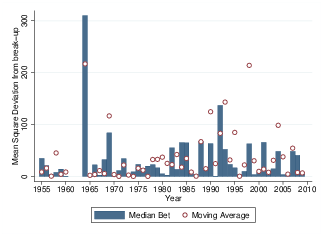
Throughout the statistical analysis the dependent variable will be the median bet in a given year. We will begin the section by asking how good the median bet is at predicting the actual outcome, as per Hypothesis 1. We will start by comparing the performance of the median bet to a series of benchmarks. We will then proceed to estimating the determinants of the median bet, to test Hypotheses 2 and 3.
We analyzed the NIC betting records from 1955 to 2009, encompassing over 10 million individual bets.6 Remarkably, the median bet by participants predicts observed ice-break-ups slightly better than our first benchmark “expert”, the historical moving average of break-up dates, although not significantly better (1-sided t-test, p=0.18, see Figure 2), with mean square deviations (MSD) from actual break-up dates of 31.06 and 35.85 respectively. This result is robust if we employ alternative metrics such as mean absolute deviation (MAD: 4.89 < 4.63, 1-sided t-test, p = 0.25).
However, when we divide the time series in pre- and post-1982 (the halfway point in the sample), the prediction of the median bet is almost significantly better than the historical moving average in the second half of the time series (MSD: 32.57 < 44.29, 1-sided t-test, p<0.09; MAD: 4.88 < 5.78, 1-sided t-test, p < 0.06).7 This improvement in performance is correlated with an increase in extreme events: looking at Figure 3, we note six years in which there were significant spikes or troughs in the time series of break-ups: 1964, 1969, 1983, 1992, 1993, and 1998. Given that most extreme events are in the second half of our sample, this would explain why the median bet’s performance relative to the moving average increases in that half of the sample, either using mean absolute deviation relative to mean square deviation. This result implies that bettors may be incorporating more information into their forecasts than just the historical record of ice break-ups.
Figure 3: Break-ups and betting on the NIC: observed break-ups (black), median bet (red). Linear time trend of break-up (slope=−0.13, t=−2.84, p<0.01, R2=0.13). Linear time trend of median bet (slope=−0.04, t=−2.93, p<0.01, R2=0.15). 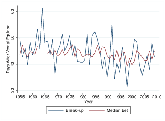
However, as Adams & Ferreira (2009) point out, in their analysis of the 2002 betting data, there are three dates (April 30th, May 5th, and May 8th), which attracted a large number of bets, since they were the most observed outcomes up to that point. In that sense, and given the relatively low number of observations in the sample, the moving average may not be the most accurate predictor, and therefore not the best benchmark of comparison. While we do not expect it to be as successful as other models, the mode is nevertheless an interesting benchmark. As such, we computed for each betting year the modal break-up day up to that point, and we compared the performance of the betting median in a given year to the contemporaneous modal break-up date. The mean square deviation of the mode was 39.24, which is significantly higher than the mean square deviation of the median bet (1-sided t-test, p = 0.03). The mean absolute deviation of the mode was 43.87, which is significantly higher than that of the median bet (1-sided t-test, p<0.01).
We also found a significant negative time trend in the median bet date (year: slope=−0.04 t=−2.91, p<0.01), in line with the negative trend in observed break-ups (year: slope=−0.07, t=−2.99, p<0.01), indicating that bettors accurately track the long-term shift in break-up. We use the linear time trend on data from 1917 up to year t to predict the ice break-up in year t+1 as another benchmark expert. Comparing the performance of that expert to our betting pool, we find no significant difference in predictive power compared to the median bet (time trend MSD = 31.61; t-test, p = 0.44; time trend MAD = 4.64, p = 0.34).
Another candidate for an expert would be someone who had access to weather data to make her predictions about the ice break-up. We consider four different experts, each with access to different information on different variables: temperature, snowfall, snow depth and precipitation. We constructed each of the four forecasts by running an OLS regression of the break-up time on the measurements of the weather variables in that year in January, February and March. We gave our experts an edge over the crowd and estimated the econometric models over the entire sample, therefore making the experts prescient about future climate conditions (though not prescient about the NIC outcome). We then compared the performance of each expert to that of the crowd. None of the experts’ performance was significantly different from that of the crowd. We attempted other models, which combined information sources (conditional on a limited number of regressors). The literature on forecasting points out that often combining forecasts can result in improved forecasting performance (Bates & Granger, 1969; Clemen, 1989; Hibon & Evgeniou, 2005). In this sense, we constructed an expert forecaster who aggregates all the aforementioned experts. We use a simple aggregation rule equal to the average; one could interpret this rule as being an expert who gives equal weight to each individual source of information. The performance of this expert was significantly worse than that of the crowd (MSD: 62.70, t=3.93, p<0.01, MAD: 6.46, t=3.19, p<0.01). The bad performance of the average forecast is clearly driven by the inclusion of the mode. Excluding the break-up mode from the average forecast leads to an improvement in performance of the “average expert”, but not enough to beat the crowd (MSD: 29.73, t=−0.41, p=0.68, MAD: 4.39, t=−0.93, p=0.36). In short, these models did not perform better than the betting pool. This constitutes our first finding.
The median bet is a reasonable predictor of the outcome of the NIC, and no worse a predictor than benchmark forecasts based on the historical distribution of break-up dates.
We now turn to what determines betting behavior and we test each of the hypotheses formulated in Section 2. Given that we have two contrasting and competing models of betting behavior, we would like to test them using the same empirical framework. The representativeness heuristic is a dynamic concept, in that it assumes recent information is more heavily weighted than other historical data, we must test it by measuring the effect of changes in recent break-up date frequencies. As such, we should also look at the change in the median bet as a result of changes in information. We will therefore employ the following econometric model:
| Δ Bt = αt + β1,t Δ Et + β2,t Δ Ht + ut (1) |
Δ Bt is the change in the median bet from year t−1 to year t. Δ Et is a vector of changes in environmental variables from year t−1 to year t. These environmental variables include as discussed before, air temperature, precipitation, snowfall and snow depth. Sagarin & Micheli (2001) find a correlation between the average air temperature, snowfall and precipitation in Fairbanks and the break-up date, which indicates there is value in using such variables as predictors of the break-up. Finally, Δ Ht is a vector of changes in history of the break-up dates. This includes changes relative to the historical average, or a proxy of the representativeness heuristic, which would be the last few years of break-ups.
Participants can collect climate and weather information in a variety of ways. On the one hand, participants experience their own local weather conditions, which they may use as information to update their beliefs about when the ice will break. On the other hand, they can find out recent trends in the weather conditions in Alaska in general, or in the vicinity of the Tanana River in particular. Participants could also either resort to media reports, or they could even contact the NIC office (Arctic Science Journeys, 1997; Seattle Times, 1986; Richards, 1995). In recent years, the NIC organizers have started providing the real-time weather conditions in the vicinity of the tripod on their website.
Figure 4: Left: Distribution of Mean March temperature (degrees Celcius). Right: Population density (people/squared kilometer). 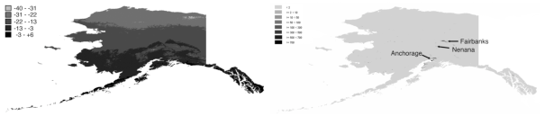
Table 1: Prais-Winsten AR(1) regression of climate determinants of betting behavior: historical break-up data.
Dep var: ΔMedian Bet (1) (2) (3) ΔMoving avg 6.235^** (2.981) 8.590^*** (3.709) 9.605^** (3.859) ΔBreakup 0.124^** (0.052) 0.153^** (0.060) ΔBreakup lag 0.069 (0.048) 0.058 (0.050) Extreme -0.617 (0.769) Extreme × ΔBreakup -0.069 (0.067) Constant 0.162 (0.207) 0.281 (0.205) 0.343 (0.231) D-W d 2.447 2.535 2.457 ρ -0.563 -0.624 -0.618 Adj. R2 0.07 0.21 0.20 Note: Rows correspond to independent variables. Regression models are numbered by column. Cell entries list regression coefficients, with standard errors in parentheses.
***, **: statistical significance at the 1% and 5% level. N=50
Therefore, when thinking about the influence of climate variables on betting, it is plausible to distinguish two possibilities. The first is that only local conditions in the Nenana area influence betting. To account for this, we collected a time series of average monthly temperature, snowfall, snow depth and precipitation in Fairbanks, which is geographically quite close to Nenana. The second possibility is that bettors may also be influenced by weather conditions in their own local area. Given we are working with the annual median bet, we do not have data on the geographic location of individual bettors, so we analyzed statewide averages. Since some areas of Alaska are much more densely populated than others and weather conditions vary widely over Alaska (see Figure 4), the weather conditions in some parts of the state will be more influential than in others. Therefore we weighed regional temperatures by the population size covered by a given weather station, using available Census data.
Table 1 describes the results of a set of Prais-Winsten regressions of historical data on changes in the median bet.8 Regression (1) looks at the effect of changes in the moving average from the previous year’s break-up: ΔMovingAvg is the difference between the historical average break-up in year t and year t−1. Hence, a positive ΔMovingAvg means last year’s break-up was later than the historical average, and the opposite is true if ΔMovingAvg is negative. We find a very large positive coefficient on ΔMovingAvg, indicating that break-ups occurring later than the historical average lead the median bet to increase.
We then augmented regression (1) to account for the effect of changes in break-up dates in the three years preceding the betting would influence betting. The variable ΔBreak-up is the difference in break-up dates in t−1 and t−2; in other words, a positive (negative) ΔBreak-up means that last year’s break-up occurred later (earlier) than the year before. ΔBreak-up Lag offers the same information regarding the years t−2 and t−3. We find a positive coefficient on both ΔBreak-up and ΔMovingAvg. However the coefficient on the latter variable is significantly larger than the former (F(1,46) = 5.30, p=0.025). In other words, the change in median bet is affected both by movements in the historical distribution and by recent shifts in break-up dates; however the former effect dominates.
We conclude this part of the analysis by asking what effect, if any, extreme events have on changes in the median bet. We construct a dummy variable, extreme, which takes a value of 1 if there was a change in break-up date of more than 10 days. Regression (3) displays the results of this augmented regression. The Extreme dummy is not significantly different from zero. As such, it is unlikely that the betting behavior is driven by behavioral biases such as the availability heuristic (Tversky & Kahneman, 1973).
Changes in the median bet are correlated with changes in the historical distribution of break-ups as well as with recent changes in break-ups.
We now turn to the question of how do bettors respond to changes in environmental conditions? Table 2 shows estimations of ΔMedian Bet on changes in environmental conditions using population-weighted Alaska-wide averages. Columns AK(1)-AK(6) display the results from different econometric specifications, which we will describe below in turn. We ran separate regressions for the effect of air temperature, snowfall, snow depth and precipitation. The reason for this is twofold: firstly, these variables are highly correlated, which would lead to collinearity problems should they be included in a single regression. Secondly, our small sample size does not permit a large number of predictors.
Table 2: Prais-Winsten AR(1) regression of determinants of betting behavior: Alaska weather data.
Dep var: ΔMedian Bet AK(1) AK(2) AK(3) AK(4) AK(5) AK(6) ΔTemp Jan -0.024 -0.058 (0.043) (0.038) ΔTemp Feb -0.062 -0.047 (0.040) (0.034) ΔTemp Mar -0.091^*** -0.079^* (0.046) (0.041) ΔSnowFall Jan -0.055 -0.054 (0.053) (0.046) ΔSnowFall Feb 0.032 0.029 (0.035) (0.032) ΔSnowFall Mar 0.096^** 0.104^** (0.045) (0.039) ΔSnowDepth Jan 0.004 (0.078) ΔSnowDepth Feb 0.026 (0.062) ΔSnowDepth Mar 0.090 (0.074) ΔPrecip Jan -0.532 (0.416) ΔPrecip Feb -0.353 (0.424) ΔPrecip Mar 0.377 (0.454) ΔMoving Avg 9.376^*** 7.488^** (3.345) (3.582) ΔBreak-up 0.124^** 0.087 (0.050) (0.052) ΔBreak-up Lag 0.070 0.093^** (0.043) (0.046) Constant -0.013 -0.007 -0.023 -0.047 0.315^* 0.259 (0.192) (0.196) (0.198) (0.200) (0.184) (0.196) D-W d 2.112 2.235 2.293 2.193 2.451 2.446 Rho -0.500 -0.490 -0.523 -0.518 -0.657 -0.590 Adj R2 0.10 0.07 0.01 0.00 0.35 0.30 Note: Rows correspond to independent variables. Regression models are numbered by column. Cell entries list regression coefficients, with standard errors in parentheses.
***, **, *: statistical significance at the 1%, 5% and 10% level. N = 50.
Regression AK(1) looks at the effect of changes in statewide air temperature averages of climate variables in the three months preceding the break-up (ΔTemp Jan, ΔTemp Feb and ΔTemp Mar). All coefficients are negative (colder winters lead to later bets), but only the March coefficient is significant. When looking at changes in snowfall in the three months preceding the break-up (ΔSnowFall Jan, ΔSnowFall Feb and ΔSnowFall Mar) in regression AK(2), we find very small and non-significant coefficients on January and February, but a positive coefficient on March—higher year-on-year snowfall in March means betting on later dates. Column AK(3) reports on the results of performing the same exercise on snow depth (ΔSnowDepth Jan, ΔSnowDepth Feb and ΔSnowDepth Mar) and column AK(4) reports on the regression with precipitation-related regressors (ΔPrecip Jan, ΔPrecip Feb and ΔPrecip Mar). We find no significant results in either case.
Regressions AK(5-6) extend the models, incorporating temperature and snowfall information respectively, to include both contemporaneous climate information and historical data. We find that introducing ΔMoving Avg—which is the change in the moving average of break-up date—to either AK(1) or AK(2) makes no difference to coefficients on the climate variables. However, the goodness-of-fit improves relative to the case where only climate information is used as a regressor.
We now perform the same exercise focusing on local conditions to the NIC, by using only Fairbanks weather station data (Table 3). The rationale for this analysis is that bettors may focus only on conditions in Nenana and ignore the climate information in their own area. Qualitatively, the results are similar to the statewide averages, with the difference that no coefficient in the regression using snowfall data is significant. We again augment the models for which we had some significant results by incorporating past break-up information. Like the analysis using AK-wide data, we find that adding ΔMoving Avg has no effect on climate coefficients but itself becomes significant vis-á-vis the case where it is the sole regressor, and it improves the goodness-of-fit, while recent changes in break-up dates remain positive and significant, while removing the significance of the ΔTemp Mar coefficient.
Table 3: Prais-Winsten AR(1) regression of determinants of betting behavior: Fairbanks weather data.
Dep var: ΔMedian Bet Fb(1) Fb(2) Fb(3) Fb(4) Fb(5) Fb(6) ΔTemp Jan -0.020 -0.040 (0.029) (0.025) ΔTemp Feb -0.027 -0.023 (0.027) (0.023) ΔTemp Mar -0.060^* -0.047 (0.033) (0.030) ΔSnowFall Jan -0.042 -0.059 (0.035) (0.031) ΔSnowFall Feb -0.009 -0.024 (0.032) (0.029) ΔSnowFall Mar 0.011 -0.001 (0.041) (0.037) ΔSnowDepth Jan 0.040 (0.069) ΔSnowDepth Feb -0.117 (0.096) ΔSnowDepth Mar 0.065 (0.079) ΔPrecip Jan -0.720 (0.511) ΔPrecip Feb 0.049 (0.657) ΔPrecip Mar -0.110 (0.203) ΔMoving Avg 9.096^** 9.398^** (3.424) (3.811) ΔBreak-up 0.129^** 0.144^** (0.050) (0.055) ΔBreak-up Lag 0.073 0.073 (0.044) (0.049) Constant 0.023 -0.013 0.014 -0.015 0.304 0.328 (0.193) (0.206) (0.204) (0.203) (0.188) (0.210) D-W d 2.808 2.298 2.750 2.323 2.506 2.546 Rho -0.520 -0.493 -0.505 -0.499 -0.653 -0.587 Adj R2 0.07 0.00 0.00 0.00 0.32 0.22 Note: Rows correspond to independent variables. Regression models are numbered by column. Cell entries list regression coefficients, with standard errors in parentheses. ***, **, *: statistical significance at the 1%, 5% and 10% level. N=50.
In short, the most influential weather variables on betting behavior are, not surprisingly, the most salient ones: temperature and snowfall. There is little to separate them in terms of their ability to explain the variance in betting. When on their own, temperature seems to outperform snowfall in terms of goodness-of-fit; however, when we include past break-up information, that difference disappears.
Another interesting comparison is between geographical sources of weather information. The AK population-weighted averages of weather variables seem to outperform local Fairbanks data in predicting the median bet. This suggests that individuals incorporate local information in their decision-making. However, we are constrained in our ability to interpret the results by the aggregate nature of our data. We therefore summarize our final finding as follows.
Historical data on break-ups and contemporaneous climate information are both good predictors of betting behavior in our sample. Weather conditions where people bet seem to matter as well as the conditions at the location of the tripod.
The Nenana Ice Classic provides a unique window into how well humans predict a naturally occurring event in the midst of a shifting climate over several decades. The NIC provides us with a time series of predictions by hundreds of thousands of Alaskans about an annual event that is highly correlated with a long-term shift in regional climate conditions.
One of the key features of the NIC is the predictions made by each of the several thousand participants are made roughly independently of each other. Participants cannot rely on any mechanism, like a market price, which provides public information—and may lead to informational cascades, or anchor beliefs about the likelihood of a given event (e.g., break-up date) taking place. As such, the distribution of bets of the NIC ought to be an accurate reflection of the bettors’ private information (and therefore beliefs) about the likelihood of the ice break-up on a given date.
Our analysis of the betting data over more than five decades finds that bettors’ predictions have changed in parallel with the historical trends of ice break up dates and broader climate changes, specifically an earlier break-up of the ice than fifty years ago. This suggests bettors incorporate the historical climate trend into their collective forecast. Furthermore, their predictions are at least as accurate as (and perhaps even slightly better than) historical models of ice break-ups, as well as models that predict the break-up of the ice using contemporaneous weather information.
We find that contemporaneous climate variables like year-to-year changes in average temperature and snowfall predict changes in betting behavior in a given year. This is quite intuitive: if this winter was colder and/or snowier than last year’s, then I ought to bet on a later date for the break-up. This seems to be true both when looking at the statewide averages (which give more weight to weather conditions where bettors reside) and when looking at conditions in the vicinity of the tripod. The fact that the regressions with AK-weighted weather variables as regressors slightly outperform the regressions with Fairbanks weather data hints at the possibility that local weather conditions to bettors who reside far from Nenana also influence betting in addition to weather conditions in the vicinity of the tripod. However, our ability to make better inference on the issue of local versus regional data sources, as well as on the causal link between climate information and betting is limited by the fact that we can analyze only aggregate data, rather than individual betting data with geographical heterogeneity.
Interestingly, we find that changes in the median bet are sensitive to changes in break-up dates in the very recent past, as well as to changes relative to the historical average. However, changes in the median bet are not sensitive to extreme events, which allows us to rule out potential mechanisms governing the crowd’s decision-making process, such as the availability heuristic. The predictive power of recent changes in break-up dates on the changes in the median bet means we cannot rule out the possibility that the crowd may be overweighing the recent past in terms of its decision-making. We cannot ascertain from our results whether the power of recent changes is due to underweighting the base rates of events, as per the representativeness heuristic, or to the discounting of past historical data as less reliable than more recent data.
This natural field experiment demonstrates that large groups can predict highly variable natural events with remarkable accuracy over a significant time span. It also suggests people do so by incorporating climate information into their decision-making. This study highlights the potential of prediction markets to tap into human perceptions of natural events. It illustrates how prediction games can be used to elicit beliefs (in the statistical sense) about the likelihood of natural events such as hurricanes (Kelly et al., 2012). They may even be used to elicit beliefs about longer-term changes to climate systems, although extended time horizons may make it difficult to make the mechanism incentive-compatible.
Importantly, prediction games can be useful tools to study what drives the formation of beliefs about climate systems. They complement the existing survey work by eliciting individuals’ beliefs about climate systems in a neutral framework, which is relatively dissociated from the political discourse around climate change.
The accuracy with which the crowd forecasted the ice break-up also hints at the applicability of such mechanisms to policy. Prediction games could be useful tools as part of disaster-prevention plans in areas of the world affected by weather phenomena.
There are, however, limitations in terms of what we can extrapolate from our data. The first limitation comes from a relative strength of this natural experiment: NIC participants are betting on a very well defined event, which has taken place over decades. As such, one would expect that participants would optimize their decision-making over time. Another limitation is that other sources of information of a social nature may influence bettors. This could include media reports: the increasing focus in the popular media about climate change may also influence betting. We leave those issues for future research.
Anderson, L.R. & Holt, C.A. (1997). Information cascades in the laboratory. American Economic Review 87, 847–862.
Adams, R. & Ferreira, D. (2009). Moderation in groups: Evidence from betting on ice break-ups in Alaska. Review of Economic Studies 77, 882–913.
Arctic Science Journeys (1997). Nenana Ice Classic. Radioscript, http://www.uaf.edu/seagrant/NewsMedia/97ASJ/04.29.97_IceClassic.html.
Armstrong, J.S. (2006). Should the forecasting process eliminate face-to-face meetings? Foresight: The International Journal of Applied Forecasting 5, 3–8.
Arrow, K.J., Forsythe, R., Gorham, M., Hahn, R., Hanson, R., Ledyard, J.O., Levmore, S. Litan, R., Milgrom, P., Nelson, F.D., Neumann, G.R., Ottaviani, M., Schelling, T.C., Shiller, R.J., Smith, V.L., Snowberg, E., Sunstein, C.R., Tetlock, P.C., Tetlock, P.E., Varian, H.R., Wolfers, J. & Zitzewitz, E. (2008). The promise of prediction markets. Science 320, 877–878.
Bates, J.M., & Granger, C.W.J. (1969). The combination of forecasts. Operational Research Quarterly 20, 451–468.
Bikhchandani, S., Hirschleifer, D. & Welch, I. (1998). Learning from the behavior of others: Conformity, fads, and informational cascades. Journal of Economic Perspectives 12, 151–170.
Bord, R. J., Fisher, A., & O’Connor, R. E. (1998). Public perceptions of global warming: United States and international perspectives. Climate Research 11, 75–84.
Clemen, R.T. (1989). Combining forecasts: A review and annotated bibliography. International Journal of Forecasting 5, 559–609.
Finkel, M. (1998). This break-up is the talk of the town when the river thaws in Nenana, Alaska, a pile of money changes hands. Sports Illustrated Magazine 88, May 18, R12.
Grether, D.M. (1992). Testing Bayes rule and the representativeness heuristic: Some experimental evidence. Journal of Economic Behavior and Organization 17, 31–57.
Hibon, M. & Evgeniou, T. (2005). To combine or not to combine: selecting among forecasts and their combinations. International Journal of Forecasting 21, 15–24.
Jorgenson, C.B., Suetens, S. & Tyran, J.-R. Predicting lotto numbers. (2011). CentER Working Paper No. 2011-033, ISSN 0924-7815.
Kelly, D., Letson, D. Nelson, F., Nolan, D. & Solis, D.. 2012. Evolution of subjective hurricane risk perceptions: A Bayesian approach. Journal of Economic Behavior and Organization 81, 644–663.
Larrick, R. P., Mannes, A. E., & Soll, J. B. (2012). The social psychology of the wisdom of crowds. In J. I. Krueger (Ed.), Frontiers in social psychology: Social judgment and decision making (pp. 227–242). New York: Psychology Press.
Larrick, R.P. & Soll, J.B. (2006). Intuitions about combining opinions: Misappreciation of the averaging principle. Management Science 52, 111–127.
Oskarsson, A.T., Van Boven, L., McClelland, G.H., & Hastie, R. (2009). What’s next? Judging sequences of binary events. Psychological Bulletin 135(2), 262–285.
Polgreen, P.M., Nelson F.D. & Neumann G.R. (2007). Use of prediction markets to forecast infectious disease activity. Clinical Infectious Diseases 44, 272–279.
Richards, B. (1995). Forget the calendar, Alaskans bet they can spot spring: This is the season for wagers on when the Tanana ice and winter will break. The Wall Street Journal April 20, A1.
Sagarin, R., & Micheli, F. (2001). Climate change in nontraditional data sets. Science 294, 811.
The Seattle Times (1986). All Bets are on ice in quest for Alaska cash. May 4, E1.
Soll, J. B., Mannes, A. E., & Larrick, R. P. (2011). The wisdom of crowds. In H. Pashler (Ed.), Encyclopedia of Mind. Sage Publications.
Suetens, S. & Tyran, J.-R. (2012). The gambler’s fallacy and gender. Journal of Economic Behavior and Organization 83, 118–124.
Surowiecki, J. (2004). The wisdom of crowds: Why the many are smarter than the few and how collective wisdom shapes business, economies, societies and nations. London: Little, Brown.
Tversky, A. & Kahneman, D. (1973). Availability: A heuristic for judging frequency and probability. Cognitive Psychology 5(1), 207–233.
Tversky, A. & Kahneman, D. (1974). Judgment under uncertainty: heuristics and biases. Science, 185, 1124–1131.
Wolfers, J., & Zitzewitz, E. (2003). Prediction markets. Journal of Economic Perspectives 18, 107–126.
Correlation coefficients on climate variables.
| ΔT | ΔT | ΔT | ΔSF | ΔSF | ΔSF | ΔSD | ΔSD | ΔSD | ΔP | ΔP | ΔP | |
| Jan | Feb | Mar | Jan | Feb | Mar | Jan | Feb | Mar | Jan | Feb | Mar | |
| ΔT Jan | 1.00 | |||||||||||
| ΔT Feb | 0.12 | 1.00 | ||||||||||
| ΔT Mar | 0.27 | 0.00 | 1.00 | |||||||||
| ΔSF Jan | -0.43 | -0.20 | -0.15 | 1.00 | ||||||||
| ΔSF Feb | -0.25 | -0.50 | -0.01 | 0.37 | 1.00 | |||||||
| ΔSF Mar | -0.26 | -0.33 | -0.56 | 0.49 | 0.52 | 1.00 | ||||||
| ΔSD Jan | -0.21 | -0.06 | 0.20 | 0.64 | 0.16 | -0.03 | 1.00 | |||||
| ΔSD Feb | -0.18 | -0.41 | 0.08 | -0.18 | 0.70 | 0.13 | -0.04 | 1.00 | ||||
| ΔSD Mar | -0.14 | -0.36 | -0.50 | 0.10 | -0.02 | 0.69 | -0.22 | -0.07 | 1.00 | |||
| ΔP Jan | 0.47 | 0.02 | 0.28 | 0.09 | -0.20 | -0.28 | 0.48 | -0.20 | -0.16 | 1.00 | ||
| ΔP Feb | 0.14 | 0.06 | 0.13 | -0.30 | 0.26 | 0.09 | -0.12 | 0.65 | -0.20 | -0.03 | 1.00 | |
| ΔP Mar | 0.19 | -0.22 | -0.10 | -0.04 | 0.07 | 0.37 | -0.14 | 0.07 | 0.58 | -0.01 | 0.05 | 1.00 |
| Note: ΔT, ΔSF, ΔSD, and ΔP denote changes in Temperature, Snow Fall, Snow Depth and Precipitation, respectively. Cell entries list correlation coefficients. | ||||||||||||
OLS regression of climate determinants of betting behavior: historical break-up data.
| Dep var: ΔMedian Bet | (1) | (2) | (3) |
| ΔMoving Avg | 5.920 (3.891) | ||
| ΔBreakup | 0.069 (0.052) | 0.107 (0.082) | |
| ΔBreakup Lag | 0.097 (0.063) | 0.084 (0.069) | |
| Extreme | −0.129 (0.103) | ||
| Extreme × ΔBreakup | −0.889 (0.893) | ||
| Constant | 0.183 (0.180) | 0.051 (0.152) | 0.078 (0.263) |
| N | 45 | 45 | 45 |
| Adj. R2 | 0.02 | 0.07 | 0.08 |
| Note: Rows correspond to independent variables. Regression models are numbered by column. Cell entries list regression coefficients, with Newey-West AR(5) standard errors in parentheses. ***, **, *: statistical significance at the 1%, 5% and 10% level. | |||
OLS regression of determinants of betting behavior: Alaska weather data.
| Dep var: ΔMedian Bet | AK(1) | AK(2) | AK(3) | AK(4) | AK(5) | AK(6) |
| ΔTemp Jan | -0.006 | -0.005 | ||||
| (0.033) | (0.037) | |||||
| ΔTemp Feb | -0.113^*** | -0.110^*** | ||||
| (0.034) | (0.033) | |||||
| ΔTemp Mar | -0.054 | -0.059 | ||||
| (0.070) | (0.067) | |||||
| ΔSnowFall Jan | -0.030 | -0.037 | ||||
| (0.058) | (0.049) | |||||
| ΔSnowFall Feb | 0.031 | 0.029 | ||||
| (0.035) | (0.030) | |||||
| ΔSnowFall Mar | 0.122^*** | 0.138^*** | ||||
| (0.043) | (0.043) | |||||
| ΔSnowDepth Jan | -0.004 | |||||
| (0.079) | ||||||
| ΔSnowDepth Feb | 0.032 | |||||
| (0.065) | ||||||
| ΔSnowDepth Mar | 0.095 | |||||
| (0.076) | ||||||
| ΔPrecip Jan | -0.030 | |||||
| (0.108) | ||||||
| ΔPrecip Feb | 0.013 | |||||
| (0.060) | ||||||
| ΔPrecip Mar | 0.090 | |||||
| (0.162) | ||||||
| ΔMoving Avg | 11.183^* | 11.135^* | ||||
| (6.402) | (5.595) | |||||
| ΔBreak-up | 0.117 | 0.135^* | ||||
| (0.081) | (0.079) | |||||
| ΔBreak-up Lag | 0.039 | 0.066 | ||||
| (0.084) | (0.064) | |||||
| Constant | 0.030 | 0.030 | 0.044 | 0.023 | 0.372 | 0.375 |
| (0.158) | (0.157) | (0.351) | (0.162) | (0.276) | (0.242) | |
| Note: Rows correspond to independent variables. Regression models are numbered by column. Cell entries list regression coefficients, with Newey-West AR(5) standard errors in parentheses. ***, **, *: statistical significance at the 1%, 5% and 10% level. N==45. | ||||||
OLS Regression of determinants of betting behavior: Fairbanks weather data.
| Dep var: ΔMedian Bet | Fb(1) | Fb(2) | Fb(3) | Fb(4) | Fb(5) | Fb(6) |
| ΔTemp Jan | -0.015 | -0.011 | ||||
| (0.030) | (0.033) | |||||
| ΔTemp Feb | -0.054^** | -0.055 | ||||
| (0.023) | (0.024) | |||||
| ΔTemp Mar | -0.035 | -0.039 | ||||
| (0.051) | (0.046) | |||||
| ΔSnowFall Jan | -0.100^*** | -0.109^*** | ||||
| (0.028) | (0.025) | |||||
| ΔSnowFall Feb | -0.061 | -0.070^** | ||||
| (0.046) | (0.031) | |||||
| ΔSnowFall Mar | 0.018 | 0.043 | ||||
| (0.035) | (0.031) | |||||
| ΔSnowDepth Jan | 0.046 | |||||
| (0.098) | ||||||
| ΔSnowDepth Feb | -0.179 | |||||
| (0.059) | ||||||
| ΔSnowDepth Mar | 0.055 | |||||
| (0.093) | ||||||
| ΔPrecip Jan | -1.500^*** | |||||
| (0.391) | ||||||
| ΔPrecip Feb | -0.977 | |||||
| (0.949) | ||||||
| ΔPrecip Mar | 0.266 | |||||
| (0.472) | ||||||
| ΔMoving Avg | 10.454 | 11.667^** | ||||
| (6.439) | (4.934) | |||||
| ΔBreak-up | 0.123 | 0.183^** | ||||
| (0.079) | (0.076) | |||||
| ΔBreak-up Lag | 0.055 | 0.057 | ||||
| (0.089) | (0.050) | |||||
| Constant | 0.032 | 0.038 | 0.045 | 0.035 | 0.356 | 0.413^** |
| (0.160) | (0.172) | (0.175) | (0.165) | (0.265) | (0.202) | |
| Note: Rows correspond to independent variables. Regression models are numbered by column. Cell entries list regression coefficients, with Newey-West AR(5) standard errors in parentheses. ***, **, *: statistical significance at the 1%, 5% and 10% level. N==45. | ||||||
Hueffer and Fonseca share lead authorship. We thank the Nenana Ice Classic staff for making lists of guesses available and Joao Madeira, Paulo Parente, Kim Peters and Margaret Short for helpful discussions. Hueffer is supported by Grant Number RR016466 from the National Center for Research Resources (NCRR), a component of the National Institutes of Health (NIH). Fonseca thanks the financial support of the University of Exeter Business School. The contents are solely the responsibility of the authors and do not necessarily represent the official view of NCRR or NIH.
Copyright: © 2013. The authors license this article under the terms of the Creative Commons Attribution 3.0 License.
This document was translated from LATEX by HEVEA.