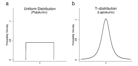
| Figure 1: Examples of a uniform distribution (platykurtic) and a non-standardized t-distribution (leptokurtic). |
Judgment and Decision Making, Vol. 8, No. 3, May 2013, pp. 330-344
Inferring uncertainty from interval estimates: Effects of alpha level and numeracyLuke F. Rinne* Michèle M. M. Mazzocco# |
Interval estimates are commonly used to descriptively communicate the degree of uncertainty in numerical values. Conventionally, low alpha levels (e.g., .05) ensure a high probability of capturing the target value between interval endpoints. Here, we test whether alpha levels and individual differences in numeracy influence distributional inferences. In the reported experiment, participants received prediction intervals for fictitious towns’ annual rainfall totals (assuming approximately normal distributions). Then, participants estimated probabilities that future totals would be captured within varying margins about the mean, indicating the approximate shapes of their inferred probability distributions. Results showed that low alpha levels (vs. moderate levels; e.g., .25) more frequently led to inferences of over-dispersed approximately normal distributions or approximately uniform distributions, reducing estimate accuracy. Highly numerate participants made more accurate estimates overall, but were more prone to inferring approximately uniform distributions. These findings have important implications for presenting interval estimates to various audiences.
Keywords: interval estimates, probability judgment, numeracy, numerical cognition, decision-making.
When the exact value of a quantity is unknown, its approximation and corresponding degree of uncertainty can be conveyed via an interval estimate—a range of possible values expected to include or "capture" the target value with a discrete probability or frequency. Researchers often present interval estimates in conjunction with formal statistical analyses (e.g., frequentist confidence intervals), and both academic and lay audiences can use interval estimates as descriptive measures of uncertainty in quantitative values. For example, prediction intervals rely on past observations (e.g., previous annual rainfall totals) to estimate the probability that some future observation (e.g., next year’s rainfall total) will fall within a given range (annual rainfall totals are roughly normally distributed in non-arid regions; Bardsley, 1984). A decision-maker (e.g., a farmer) may combine this information with an implicit or explicit assumption of normality to gain a sense of the probability distribution of future outcomes.
An important feature of interval estimates is their alpha level—the probability or frequency with which the target value is expected to fall outside the interval. Alpha levels typically equal .10 or .05, respectively reflecting 90% or 95% certainty or reliability (i.e., confidence) of capturing the target quantity within the interval. This convention derives from the norms of statistical hypothesis testing established by Fisher (1925). Statistical results are deemed "significant" if there is a low probability (p < .05 or p < .10) that similar or more extreme results would arise at random. Conventional alpha levels of .05 or .10 are commonly used for interval estimates related to everything from political polls (Hillygus, 2011) to blood test results (Armitage, Berry, & Matthews, 2002) and are pervasive in academic publishing.
What is the basis for choosing a particular alpha level? Are .05 or .10 alpha levels appropriate in all contexts, or should different alpha values be used, particularly when interval estimates serve a descriptive purpose? What alpha level is appropriate for interval estimates used in everyday life, outside the context of scientific research? What alpha level is best for the rainfall prediction interval presented to the aforementioned farmer? Questions like these pose a challenge, because the range of relevant values and the degree of certainty required may differ across situations (e.g., what crop the farmer raises, its drought tolerance, etc.). In addition, individuals may differ in how they interpret interval estimates. Ideally, probabilistic inferences drawn from interval estimates should be relatively accurate and consistent across individuals and contexts. In many situations, it is impractical to present highly detailed information about probability distributions (e.g., quintiles, graphs, etc.), so, if possible, interval estimates should accurately convey not just the probability that an outcome will fall outside a given pair of endpoints but also the approximate overall shape of the probability distribution. To our knowledge, no research has investigated how interval estimate alpha levels affect the accuracy of distributional inferences. In this paper, we address this question by examining how the alpha levels of prediction intervals influence capture probability estimates for varying ranges. We also evaluate the effects of numerical and mathematical ability, or numeracy, on the accuracy of capture probability estimates and the approximate shapes of inferred probability distributions.
In the reported experiment, participants received information about prediction intervals for future annual rainfall totals in each of several fictitious cities. These prediction intervals differed in alpha level but consistently implied normal distributions with the same amount of variability (i.e., the standard deviation of the implied distribution was held constant to control for the actual amount of uncertainty present). Participants then estimated probabilities that next year’s rainfall total would be captured within three different ranges about the mean. Collectively, these estimates provided a cross-sectional view of the probability distribution inferred from each prediction interval, allowing us to reconstruct the approximate shapes of these inferred distributions. Our aim was to evaluate whether alpha levels affect the accuracy of distributional inferences, as well as whether accuracy or any observed effects on accuracy vary with numeracy skills.
There is an existing literature on the formulation of subjective interval estimates—interval estimates people create for unknown values based on their degree of certainty in their own judgment (e.g., Juslin, Wennerholm, & Olsson, 1999; Juslin, Winman, & Hansson, 2007; Klayman, Soll, Gonzalez-Vallejo, & Barlas, 1999; Soll & Klayman, 2004; Winman, Hansson, & Juslin, 2004). Unlike the present study, participants in studies of subjective interval estimation provide their own estimates of quantities (e.g., prices, dates, distances, etc.) and determine their own interval endpoints and/or confidence levels. Researchers then analyze whether these subjective interval estimates capture actual values as often as would be implied by average confidence levels. The alignment of subjective confidence with actual capture probabilities is often termed the "calibration" of judgment. A common finding in calibration research is that subjective interval estimates tend to capture the true value at a rate well below individuals’ average confidence levels—that is, participants are often overconfident (e.g., Soll & Klayman, 2004).
Of potential relevance to the present study is research by Teigen and Jorgensen (2005) on how people’s confidence levels in subjective interval estimates relate to interval widths. Teigen and Jorgensen asked participants to create intervals that would capture an unknown quantity’s value (e.g., the population of Spain) with a given confidence level (e.g., 90%). However, those same participants subsequently estimated that the intervals they created would actually capture the target value at a much lower rate (e.g., 50%), indicating a form of overconfidence in the original interval estimate. Although this result could be taken to suggest that people believe interval estimates generally capture target values at a rate lower than that indicated by the assigned level of confidence, subjective interval estimation is quite different from cases in which complete interval estimates are presented as objective sources of information about the approximate value of a quantity. The findings of Teigen and Jorgensen do not mean that people think interval estimates they receive as information are poorly calibrated—or that people will necessarily infer distributions that are different from the one implied by that information. If we consider the example of annual rainfall totals, Teigen and Jorgensen’s work is relevant to the question of how people would use their own prior knowledge (e.g., of weather patterns) to relate capture probability to a range of possible rainfall totals. This is an issue of the calibration of subjective judgment. In contrast, the present study investigates how people use information about the likelihood of the rainfall total falling within a given range to infer a probability distribution and assess the chances of the total falling within different ranges. This is an issue not of calibration, but of the proper interpretation of quantitative information.
Figure 1: Examples of a uniform distribution (platykurtic) and a non-standardized t-distribution (leptokurtic).
The notion of "bounded rationality" (e.g., Simon, 1957) is consistent with the idea that people likely utilize descriptive prediction intervals in a relatively intuitive, heuristic manner of the sort described by Tversky and Kahneman (1974). For example, imagine that the farmer receives a rainfall prediction interval with an alpha level of .05, indicating a 95% probability that next year’s total will fall within 12 inches of the annual average. What may matter most to the farmer is not the probability that the total will fall within 12 inches of the mean, but rather the probability that the total will fall within 6 inches of the mean, as values outside this narrower range will damage the crop. To determine this latter probability, the farmer may (either explicitly or implicitly) compare the sizes of the two ranges (±6 in. vs. ±12 in.) and intuitively adjust the confidence level accordingly. Whether or not this would lead to accurate inferences of uncertainty is unclear. On the one hand, Griffiths and Tenenbaum (2006) showed that individuals possess accurate implicit probabilistic models of everyday phenomena and can use these models effectively to make intuitive predictions about future outcomes. On the other hand, heuristic reasoning sometimes leads to non-normative interpretations of descriptive statistical information (e.g., boxplots; Lem, Onghena, Verschaffel, & Van Dooren, in press).
Even if an individual recognizes (implicitly or explicitly) that annual rainfall totals tend to be normally distributed, the alpha level that serves as the starting point for adjustment could potentially affect the shape of the inferred distribution. Low-alpha prediction intervals (e.g., α = .05) exclude only very rare outcomes; interval endpoints lie in the distribution’s tails, far from the mean. In the tails, the slope of the normal curve approaches zero, so incremental movements of interval endpoints affect capture probability only slightly. Narrowing the interval the farmer receives (a ±12 inch range about the mean) by two inches per side (a 17% reduction in width) only reduces capture probability from 95% to 90%, which may be counterintuitive. Individuals’ experiences with stochastic phenomena naturally tend to involve relatively common outcomes near the center of the distribution (e.g., rainfall totals close to the mean), where the size of the relevant range about the mean has a much steeper effect on capture probability. Thus, receiving wide, low-alpha interval estimates may lead to downward over-adjustments of capture probability for narrower ranges, consistent with the inference of an "over-dispersed" normal probability distribution (i.e., a larger standard deviation than is implied by the interval estimate).
Low alpha levels could also lead to capture probability estimates that are consistent with a non-normal distribution. This could result from a misconception about the relevant probabilistic model, or from systematic inaccuracies in estimation, despite some sense that the distribution is normal. If estimated capture probability decreases with interval width too quickly, a platykurtic, or "boxy" distribution may provide a better fit to estimates than a normal distribution, a possibility we consider in the present study. The uniform distribution (Figure 1a) represents the extreme case—one in which there is no central tendency, as capture probability decreases linearly with interval width. Capture probabilities that decrease with interval width faster than a linear function would result in a bimodal probability distribution, a possibility we do not consider, as it seems highly implausible that an individual would infer a bimodal distribution from an interval estimate (nor would it be sensible to present an interval estimate for a bimodal distribution).
Our primary hypothesis is that presenting interval estimates with low alpha levels may lead to capture probability estimates that are fit best by over-dispersed normal distributions or non-normal platykurtic distributions. However, in some cases, participants may infer an under-dispersed normal distribution or a non-normal leptokurtic distribution (i.e., a distribution that is "pointy" compared to the normal distribution). In this case, participants’ capture probability estimates may fit better with a non-standardized t-distribution1 (Figure 1b) than a normal distribution. Although we did not hypothesize that specific alpha levels or participant characteristics would lead to inferences of leptokurtic distributions, we considered this potential shape in the interest of completeness and for exploratory purposes.
Ultimately, the use of certain alpha levels may lead more consistently to capture probability estimates that fit well with the appropriate normal distribution. Such a result would point toward alpha levels that may be preferable when descriptive interval estimates will be used to draw intuitive distributional inferences. Although it might be possible in such cases to explicitly inform individuals that the relevant distribution is normal in form, this will be impractical unless the recipient of the interval estimate has at least a basic knowledge of probability theory. For the general population (e.g., patients in health care settings, consumers of weather information, etc.), such knowledge is probably not the norm. In addition, it is interesting from a theoretical perspective to consider the inferences people draw based on their intuitive probabilistic models of the phenomenon in question. Thus, we chose not to provide the participants in our study with any explicit information about the relevant distributional form, but chose a domain (annual rainfall totals) for which a normal distribution is relatively intuitive.
Of secondary interest in this study was our hypothesis that people with low numeracy may exhibit poorer capture probability estimates and may be more prone to inferring incorrect distribution shapes in response to interval estimates. We base this hypothesis on evidence that numeracy varies widely, even among educated adults (Lipkus, Samsa, & Rimer, 2001), with individual differences influencing intuitive numerical judgments and everyday decisions, even when explicit calculation is not required (Reyna, Nelson, Han, & Dieckmann, 2009). For example, people with lower numeracy are more susceptible to framing effects due to numerical format (e.g., frequency vs. probability; Peters et al., 2006). Moreover, a central aspect of numeracy involves the precision of people’s mental representations of numerical magnitude (Dehaene, 2011). Those with more precise numerical representations not only tend to exhibit greater mathematical ability (Halberda, Mazzocco, & Feigenson, 2008), but are also more strongly influenced by relevant proportional differences during decision-making (Peters, Slovic, Västfjäll, & Mertz, 2008). Therefore, we suspect that individual differences in numeracy may affect people’s use of interval estimates to draw inferences about probability distributions. In the experiment described below, we evaluated numeracy via a brief test of numerical skills and also asked participants whether they had taken any formal statistics classes.
The research undertaken in this study is novel and important for several reasons: First, to our knowledge, no one has investigated whether the alpha levels of interval estimates presented as information affect the probability distributions people intuitively infer. The answer to this question has practical applications in terms of the presentation of interval estimates to various audiences, and it may also have implications for theoretical questions regarding the accuracy of implicit probabilistic models. Second, the methodology we have developed—specifically, our method of reconstructing inferred probability distributions from a series of capture probability estimates—could potentially be applied in a wide variety of research settings to assess beliefs about probability distributions. Finally, our study extends the existing literature on numeracy by considering how numeracy affects the interpretation of interval estimates, a form of quantitative information that has not yet received much attention in this regard.
A total of 200 students in psychology courses at a large, top-tier public university were recruited (M age=20.2; 75 males). Students earned course credit for completing a series of paper-and-pencil experiments; the present experiment was the first in the series. Before beginning, participants were told they would be making quick, intuitive probability estimates in less than 15-20 seconds (this instruction effectively discouraged attempts to calculate answers).
Participants completed four trials. During each trial, participants received the mean annual rainfall total (in inches) for a fictitious town, along with a prediction interval for future totals. The alpha level of the prediction interval differed across trials (.05, .10, .25, and .40), but corresponding interval widths were set such that all prediction intervals implied approximately the same normal distribution (SD≈6; hereafter referred to as the "implied" distribution).
After receiving information about a given prediction interval, participants were asked to judge the probabilities that next year’s rainfall total will fall within ±3, ±6, and ±9 inches of the mean. These ranges were chosen to reflect a cross-section of the probability distribution, allowing us to obtain data on the participant’s impression of the distribution’s overall shape. Thus, participants gave capture probability estimates for the three different range sizes in response to prediction intervals with each of the four alpha levels, for a total of 12 estimates. Regardless of the alpha level, the assumption of a normal distribution implies capture probabilities of approximately .38, .68, and .86 for the ±3, ±6, and ±9 inch ranges, respectively.
After completing all four trials, participants performed additional tasks not relevant to this study, with the exception of one survey item about statistics coursework and a ten-item timed (ten-minute) math test. Finally, participants were debriefed on the purpose of the experiment and provided with the normative responses to estimation and test items.
For each of the four trials, participants were given one sheet of paper (see supplemental materials). At the top, a prediction interval was presented in a short paragraph, such as the following (bolding/underlining included):
Historical data indicates that the average annual rainfall total in Grand Prairie is 30 inches, and there is a 95% chance that any given year’s total will be within 12 inches of this average (i.e., a 95% chance that the total will be between 18 inches and 42 inches).
Participants read this paragraph silently. Below, three separate prompts asked participants to estimate the probabilities that next year’s annual total will fall within different margins of the annual average (±3, ±6, or ±9 in.). The following is a sample prompt:
What do you think is the probability that next year’s rainfall total will be within 3 inches of the average (i.e., between 27 inches and 33 inches)?
%
Participants estimated capture probabilities in either ascending or descending order with respect to range size (i.e., ±3, ±6, then ±9 in. or ±9, ±6, then ±3 in.). This order was randomly assigned for each participant and held constant across trials to minimize confusion. The presentation order of prediction intervals with different alpha levels (.05, .10, .25, or .40) was counterbalanced based on a 4 × 4 Latin square. Four different counterbalanced orderings of town names (Grand Prairie, Townsville, Cedar Hills, or Brook Hollow) and rainfall means (25, 30, 35, or 40 in.) were created and randomly assigned to participants. Although no explicit information about the probability distribution of rainfall totals was presented, the fact that the means were exactly at the center of the interval estimates is suggestive of a symmetric, unimodal distribution.
A survey item included in this study asked participants to report (yes/no) whether they ever had taken a statistics course (level not specified). The math test was designed to measure variability in general numeracy skills among college students. There were ten items on assorted topics (e.g., place value, counting, probability, percent change, or average/median; see supplemental materials). These items were presented in a fixed order across participants, roughly in order of increasing difficulty. Math test scores reflect the number of correct responses (out of 10) achieved within the 10-minute time limit.
Six participants (3 male; 3% of the total sample) were excluded because of incomplete or incoherent responses. Responses were considered incoherent if the judged capture probability for a smaller range (e.g., ±3 in.) equaled or exceeded that for a larger range (e.g., ±6 in.). Such responses suggest a misunderstanding of either the task or the concept of probability. The remaining 194 participants were included in all subsequent analyses, which we present below in three sections. First, to investigate how capture probability estimates were affected by experimental manipulations and covariates, we conducted an ANCOVA and related post-hoc analyses. Next, we analyzed the approximate shapes of the probability distributions participants inferred, using regression analyses to fit different distribution forms (normal, t-distribution, and uniform) to participants’ capture probability estimates. In the third section of results, we present several analyses that focus specifically on effects of numeracy.
The raw error in participants’ estimates of capture probability (estimated−actual) differed depending on both of the main experimental factors—alpha level and range size—and was also influenced by individual differences in numeracy. We conducted a repeated-measures ANCOVA with two within-subjects factors: a) the alpha level (Alpha: .05, .10, .25, .40), and b) the range for which capture probability was estimated (Range: ±3, ±6, or ±9 in. about the mean). Between-subjects factors included the presentation orders of different alpha levels, range conditions, town names, and mean rainfall totals. Prior statistics coursework was a binary factor, and the centered math score (# correct−mean) was a covariate.
Figure 2: Mean error in capture probability estimates, by alpha level of prediction interval presented and size of the range for which capture probability was estimated. Error bars indicate the standard error of the mean within each condition (un-pooled variances). 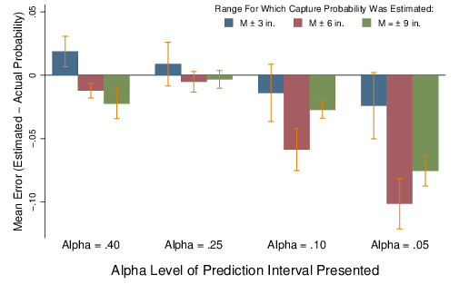
There were no significant effects of presentation order for alpha levels (p=.149), town names (p=.673), or rainfall means, (p=.638). The order in which estimates were made for different range sizes (ascending vs. descending) had a small but statistically significant effect on error (Mascend=−.001, Mdescend=−.015), F(1,179)=5.453, p=.021, ηp2=.030.
Mauchly’s test of sphericity indicated that variances differed across levels of Alpha, W(5)=.333, p<.001, Range, W(2)=.354, p<.001, and the Alpha × Range interaction, W(20)=.461, p<.001. Therefore, the Greenhouse-Geisser correction was applied for all results involving within-subjects factors. There were significant main effects of Alpha, F(1.823,326.290)=16.414, p<.001, ηp2=.084, and Range, F(1.215,217.506)=23.876, p<.001, ηp2=.118. The Alpha × Range interaction was also significant, F(4.770,853.752)=5.537, p<.001, ηp2=.030.
Overall, capture probability estimates were relatively accurate for moderate alpha levels (.40 or .25), but were relativley inaccurate for low alpha levels (.10 and .05; see Figure 2). Low alpha levels led participants to significantly underestimate capture probabilities, particularly for the ±6 and ±9 inch ranges.
As seen in Figure 2, accuracy was not necessarily improved when the endpoints of the prediction interval presented were close to the endpoints of the range for which capture probability was estimated. A prediction interval with an alpha level of .10 covers ±10 inches about the mean, but for the ±9 inch range, estimates were actually better when prediction intervals covered ±5 inches (α=.40) or ±7 inches (α=.25) about the mean. In addition, for the ±3 inch range, estimate error only differed significantly from zero when participants received the prediction interval with the closest set of endpoints (±5 inches, α=.40).
Note that for low alpha levels, underestimation increases with the move from the ±3 inch range to the ±6 inch range, but then declines with the move from the ±6 inch range to the ±9 inch range. A post-hoc trend analysis confirmed the presence of a significant quadratic component in the main effect of Range, F(1,179)=84.886, p<.001, ηp2=.322. This trend suggests a tendency to infer over-dispersed distributions—either normal distributions with larger-than-appropriate standard devations, or platykurtic ("boxy") distributional forms. Such distributions have lower probability density at the peak compared to the implied normal distribution. Thus, negative error in capture probability estimates rises as the range initially increases from zero, but this increase continues only until the two distributions intersect. Flatter or boxier distributions have larger tail probabilities, so once the inferred and implied distributions cross, the error shrinks back to zero, leading to the observed quadratic relationship. The results found here suggest that for low alpha levels, the x-values where the implied and typical inferred distributions intersect—at which point the difference in capture probability for a given range reaches its maximum—may lie relatively close to ±6 inches about the mean rainfall total.
Error in capture probability estimates was not related to self-reported statistics coursework (p=.327). Math score (Mean=6.40, Median=6, SD=2.24) had a significant effect on estimate accuracy, but in the opposite direction of predictions—higher math scores were associated with more error in the negative direction, not less, F(1,179)=7.096, p=.008, ηp2=.038. There was also a significant quadratic trend in the negative effect of math scores on error, F(1,179)=6.021, p=.015, ηp2=.033. Additional analyses related to the effect of math score on error will be presented in Section 3.3, which focuses on numeracy effects.
There was a significant interaction between range size and the order of estimation prompts (ascending vs. descending range size), F(1.215, 217.506) = 6.512, p = .008, ηp2= .035. Participants who estimated capture probabilities for ranges of descending size (±9, ±6, then ±3 inch range) exhibited positive error for the ±3 inch range (Mdescend=.021 vs. Mascend=−.023), rather than the typical negative error observed in other conditions.
The centered math score interacted significantly with both Alpha, F(1.823, 326.290) = 5.583, p = .005, ηp2=.030, and Range, F(1.215, 217.506) = 13.010, p < .001, ηp2= .068. The main effect of Alpha on capture probability estimate error (increased negative error for low alpha levels vs. moderate alpha levels) was roughly twice as large for participants with the highest math scores (8-10; Mlow-α=−.078 vs. Mmod-α = .008) compared to other participants (0-7; Mlow-α=−.035 vs. Mmod-α = .0002). Meanwhile, there was a significant negative correlation between math scores and estimation error for the ±3 inch range, r = −.156, p = .030, an almost significant positive correlation for the ±9 inch range, r = .132, p = .067, and no significant correlation for the ±6 inch range, r = −.096, p = .186. Further analyses relevant to observed interactions involving math scores will be presented later in the section on numeracy effects.
Although the ANCOVA results presented in the previous section show that error in capture probability estimates varies with alpha level and numeracy, this does not reveal what distributional shapes fit best with participants’ capture probability estimates within each alpha level. Therefore, we conducted a series of regression analyses to investigate how alpha levels influence the distributional shapes participants inferred from the interval estimates they received. In general, these regression analyses show that the type of distribution that best fit participants’ estimates is strongly dependent on the alpha level of the prediction interval presented, but there is also considerable variation between individuals.
For each set of three capture probability estimates (±3, ±6, or ±9 inches about the mean) that a given participant made in response to a prediction interval with a given alpha level (.40, .25, .10, or .05), we constructed three different regression models. Each model assessed the fit of a different distributional form: a normal distribution, a non-standardized t-distribution (leptokurtic), or a uniform distribution (platykurtic). We fit normal and t-distributions using nonlinear regression. We used linear regression to fit uniform distributions, as this distributional form implies that capture probability decreases linearly with the width of the interval.
For the regression analyses, it was assumed that the means of all inferred distributions were zero, which makes the upper bound of the interval for which capture probability was estimated—denoted here by x—equal to 3, 6, or 9 inches, depending on the range condition. The regression equations used to model participants’ estimates in terms of each distribution type are defined here in terms of the cumulative distribution function (CDF), FX(x)=P(X ≤ x), for a random variable X with the specified probability distribution2. Because the intervals for which capture probability was estimated are symmetric about the mean (excluding equivalent lower-tail and upper-tail regions), capture probability estimates were modeled as follows:
| (1) |
Assuming that distributions are centered (M = 0), both the normal and uniform probability distributions (and their CDFs) are defined by a single parameter. For the normal distribution, this parameter is the standard deviation. We define uniform distributions based on their "width", the difference between the highest and lowest outcome values with non-zero probability (alternatively, the uniform distribution can be defined by its "height", the probability density for any possible outcome). In contrast, the centered t-distribution is defined using two parameters—a scaling parameter that controls the spread, and a second parameter that corresponds to the number of degrees of freedom (df) when the t-distribution is used to model a sample of values drawn from a normal population. However, for our purposes, the df parameter simply controls how heavy the tails of the distribution are.
Table 1: Counts of best-fitting distribution types, by alpha level of the interval estimate presented and the type of distribution that best fit capture probability estimates.
Distribution Type α Normal T-dist. Uniform Total .40 79 83 32 194 .25 78 68 48 194 .10 54 55 85 194 .05 38 62 94 194 Total 249 268 259 776
We assessed the fit of each set of three capture probability estimates with each of the different distribution types by examining adjusted-R2 values for the three regression models:
| Adj R2=1− | ⎛ ⎜ ⎜ ⎝ |
| ⎞ ⎟ ⎟ ⎠ | ⎛ ⎜ ⎜ ⎝ |
| ⎞ ⎟ ⎟ ⎠ | (2) |
Table 2: Mixed-effects multinomial logistic regression model of best-fitting distribution type.
Outcome Predictor OR SE z p 4*23mmT-dist. Fits Best (vs. Normal) Math Score 0.827 0.058 -2.69 0.007 α=.25 0.693 0.187 -1.36 0.175 α=.10 0.657 0.194 -1.42 0.155 α=.05 1.123 0.342 0.38 0.704 4*26mmUniform Fits Best (vs. Normal) Math Score 1.071 0.063 1.17 0.244 α=.25 1.732 0.524 1.81 0.070 α=.10 5.568 1.719 5.56 < 0.001 α=.05 9.070 2.940 6.80 < 0.001
The model with the highest adjusted-R2 value was considered the "best-fitting" distribution. Adjusted-R2 takes into account the number of explanatory terms in the model, which is important, because the centered t-distribution was fit using two free parameters, while there is only one free parameter for centered normal and centered uniform distributions. A t-distribution should only be seen as providing the best fit with participants’ responses if the corresponding regression model increases the R2 value more than would be expected by chance with the introduction of a second explanatory term.
Table 1 shows counts of the different distribution types that best fit participants’ capture probability estimates for each alpha level. Because regression models were fit to only three data points, results should be interpreted with some caution. R2 values were generally high (>.90) for all three distribution-type models, and in many cases, increases in explanatory power associated with one model over another were small. Thus, classifications of participants’ responses according to distribution shape are likely somewhat "noisy" and may be relatively arbitrary in borderline cases. However, when viewed in aggregate, the results provide a good deal of information about the effect of alpha level on the approximate shapes of the distributions that participants inferred.
As seen in Table 1, participants’ estimates were fit best by a normal distribution considerably more often when alpha levels were moderate (.40 or .25) rather than low (.10 or .05). Low alpha levels increased the frequency with which estimates were fit best by a uniform distribution, reducing the frequencies of best-fitting normal and t-distributions. The results described in Table 1 were corroborated by a mixed-effects multinomial logistic regression analysis. A model was constructed to predict how the best-fitting distribution for each set of estimates varies according to the alpha level and participant. Fixed effects included dummy variables for alpha levels, as well as each participant’s centered math score. Random intercepts accounted for additional within-subject regularities in best-fitting distribution shape. The base outcome was that a normal distribution provided the best fit. The .40 alpha level was the reference group for effects of alpha level. Table 2 gives the parameter estimates for the model in terms of odds ratios (OR), which measure the extent to which each predictor increases the odds that a t-distribution or uniform distribution, respectively, fits estimates better than a normal distribution.
Table 3: Average parameter values of best-fitting distributions, by alpha level of the prediction interval presented and type of distribution that best fit estimates.
Best-Fitting Distribution Type T-dist. α df Scale .40 2.50 3.60 .25 2.10 3.47 .10 1.86 2.69 .05 1.27 2.65
The alpha level was not significantly associated with the odds of inferring a t-distribution (leptokurtic) rather than a normal distribution. However, successively lower alpha levels dramatically increased the odds that estimates were fit best by a uniform distribution (platykurtic). Also, higher math scores significantly decreased the odds that a t-distribution provided a better fit than a normal distribution, but there was no analogous effect for the uniform distribution. This indicates that higher math scores were associated with higher best-fit frequencies for both normal and uniform distributions compared to t-distributions.
Figure 3: Average probability distributions (distributions with average parameter values), by best fitting distribution type (frequency = n) and alpha level. 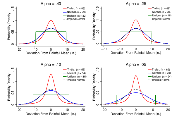
Table 4: Mean error in capture probability percent estimates, by best-fitting distribution type, alpha level, and range size (±3, ±6, or ±9 in.).
α=.40 α=.25 Best Fit ±3 ±6 ±9 ±3 ±6 ±9 Normal -0.07 0.32 1.50 -1.09 -0.02 -0.59 T-dist. 7.07 -2.63 -8.91 12.05 1.50 -3.22 Uniform -6.83 -1.34 5.90 -11.74 -4.15 4.21 α=.10 α=.05 Best Fit ±3 ±6 ±9 ±3 ±6 ±9 Normal -3.18 -2.58 -3.16 -5.95 -9.51 -10.19 T-dist. 18.70 4.84 -1.63 19.61 5.05 -2.23 Uniform -13.25 -14.88 -3.16 -15.48 -20.40 -9.97
In addition to considering what types of distributions provided the best fit to participants’ capture probability estimates, it is also important to consider the parameter values of these best-fitting distributions. A participant could potentially draw the proper inference of a normal distribution, but yet be so far off with respect to the standard deviation that associated capture probability estimates are quite poor—perhaps poorer, even, than estimates derived from a non-normal inferred distribution with the right parameter value(s). To determine the typical values of distribution parameters, we calculated the average parameter values of participants’ best-fitting distributions within each distribution classification (Table 3).
As Table 3 shows, the values of each parameter appear to be related to the alpha level of the prediction interval presented. To verify, we conducted post-hoc tests for monotonic trend in the parameter values of best-fitting distributions as alpha levels decreased. For best-fitting normal distributions, there was a positive monotonic trend in the standard deviation, z = 8.24, p < .001. For best fitting t-distributions, there was a marginally significant negative trend in the df parameter, z = −1.67, p = .094, and a significant negative trend in the scale parameter, z = −4.39, p < .001. There was also a significant positive trend in the width of best-fitting uniform distributions, z = 11.85, p < .001. It is important to keep in mind, however, that these are not trends within individuals, as the type of distribution that best fit a given participant’s estimates often changed with the alpha level.
Figure 3 shows graphs of probability distributions with the average parameter values from Table 3, along with the number of participants in each condition whose estimates were fit best by that distribution type. Although "wisdom of the crowd" effects (e.g., Galton, 1907) may be at play here, visual inspection of the figure suggests that best-fitting normal distributions were very close to the implied normal distribution (though the similarity declines a bit for lower alpha levels, particularly the .05 level). This result suggests that inferring the proper (normal) distributional form may be an important factor in making accurate capture probability estimates.
Table 5: Mixed-effects linear regression model of error in capture probability estimates.
Predictor B SE z p Math Score 0.026 0.115 0.230 0.882 Low Alpha -5.279 0.748 -7.060 < 0.001 T-dist. Fits Best 0.144 0.671 0.210 0.830 Uniform Fits Best -2.225 0.804 -2.770 0.006 Low Alpha × T-dist. Fits Best 11.940 1.036 11.530 < 0.001 Low Apha × Uniform Fits Best -5.409 1.086 -4.980 < 0.001 Constant 0.148 0.483 0.310 0.760
Table 4 gives the mean estimation error associated with best-fitting distribution shapes, broken down by both alpha level and range size. Several trends are apparent. First, at alpha levels other than .05, estimates that were fit best by a normal distribution are quite accurate. Also, as would be expected given the shapes of the uniform distribution (platykurtic) and t-distribution (leptokurtic), the direction of error in estimates best fit by these distributions appears to be related to the range for which capture probability was estimated. The best-fitting t-distributions tended to have high peaks and a strong central tendency, reflecting overestimation of capture probability, particularly for narrower ranges. The reverse is true for participants whose estimates were fit best by a uniform distribution. Probability density is relatively low and even across the entire distribution, reflecting increasing underestimation of capture probability as the range narrowed.
It also appears in Table 4 that the strength of the trends described above increases for lower alpha values (.05 and .10). Again, however, bear in mind that the type of distribution that tended to fit best was also dependent on the alpha level, so the means in Table 4 should not be taken to indicate the overall effects of alpha level. Nonetheless, it is interesting to note that, as suggested by Figure 3, low alpha levels decreased the accuracy of capture probability estimates that were fit best by a normal distribution. In addition, estimates that were fit best by non-normal distributions (uniform or t-distributions) were also poorer in low-alpha conditions than in high-alpha conditions.
The apparent trends just described are indeed statistically significant. We conducted a mixed-effects linear regression to model error in capture probability estimates, which, for each participant, were averaged across the three range conditions for each alpha level. As before, potential within-subject regularities were modeled via random intercepts, and the math score was a fixed predictor. For this analysis, we condensed the four alpha levels into two groups: low alpha levels (.05 and .10) and moderate alpha levels (.25 and .40). This makes interpretation simpler, as we also modeled the interaction of alpha level and best-fitting distribution type to verify whether trends associated with each distribution type indeed become stronger with lower alpha levels. The more detailed model (with three alpha level predictors and six interaction terms) shows essentially the same results as the model presented in Table 5.
The Low Alpha × Uniform Fits Best interaction does have a significant effect on the average estimation error, indicating that low alpha levels exacerbate the tendency for estimates best fit by uniform distributions to be too low for smaller ranges. This effect can be seen in Figure 3 in the graph for the two lowest alpha levels (.05 and .10), as the "heights" of the average best-fitting uniform distributions are lower compared to those for moderate alpha levels (.25 and .40). Meanwhile, the significant Low Alpha × T-dist. Fits Best interaction indicates that the reverse tendency for estimates best fit by t-distributions to be too high is also stronger when alpha levels are low. This is reflected in Figure 3 by the fact that the t-distributions were "pointier" (more leptokurtic) when prediction interval alpha levels equaled .05 or .10. Thus, we can see that low alpha levels not only increase the likelihood of inferring a non-normal probability distribution, but also make the non-normality of these inferred distributions more extreme.
Overall, the regression analyses we conducted support the earlier finding that capture probability estimates were most accurate when alpha levels were moderate (.25 or .40). Additionally, the results show that the accuracy of capture probability estimates was associated with the inference of an approximately normal distribution shape. Thus, it appears that moderate alpha levels improved capture probability estimates not only by supporting the inference of the correct distributional form, but also by improving the accuracy of estimates regardless of which distributional form fit participants’ estimates best. Finally, it is interesting to note that the math score is no longer significant in the regression model of estimation error shown in Table 5. This suggests that the relationship between math scores and estimation error seen earlier in the ANCOVA (greater negative error with higher scores) arises largely due to the effect of numeracy on the form of the inferred distribution, rather than effects on parameter values. We now explore results related to numeracy in more detail.
A closer analysis of the role of numeracy shows that higher math scores had both positive and negative effects on the accuracy of capture probability estimates. The ANCOVA described earlier primarily showed the negative effect. An initial indication as to the origin of this effect comes from the regression model presented in Table 2: Higher math scores were related to decreasing chances of a t-distribution fitting estimates better than a normal distribution, but did not affect the chances of a uniform distribution fitting better than a normal distribution. Thus, while higher math scores do appear to increase the likelihood of inferring an approximately normal distribution shape (rather than a t-distribution), they also increase the chance of inferring an approximately uniform distribution shape. The negative effect of numeracy arises because estimates were least accurate when approximately uniform distributions were inferred, particularly when alpha levels were low (see Table 4).
Table 6: Proportions (counts) of best-fitting distribution type, by math score group and alpha level, with group sizes (n) and chi-squared tests of association.
α=.40 α=.25 α=.10 α=.05 Math Group N T U N T U N T U N T U Low (0-4) 35% 54% 11% 38% 35% 27% 19% 32% 49% 24% 41% 35% (n = 37) (13) (20) (4) (14) (13) (10) (7) (12) (18) (9) (15) (13) Middle (5-7) 39% 49% 12% 36% 43% 21% 30% 37% 33% 13% 36% 51% (n = 90) (35) (44) (11) (32) (39) (19) (27) (33) (30) (12) (32) (46) High (6-10) 46% 28% 25% 48% 24% 28% 30% 15% 55% 25% 22% 52% (n = 67) (31) (19) (17) (32) (16) (19) (20) (10) (37) (17) (15) (35) χ2(4)=10.93 χ2(4)=6.55 χ2(4)=12.42 χ2(4)=8.19 p=0.027 p=0.161 p=0.015 p=0.085 Note: N = normal distribution, T = t-distribution, U = uniform distribution.
To further explore the effects of numeracy and consider the role of prediction interval alpha levels, we classified participants’ math test scores into three groups. The "middle" group (5-7) included scores within one of the median (6), while the "high" and "low" groups included scores above 7 and below 5, respectively. Then, for each alpha level, we constructed a contingency table relating math score group to the distribution type that best fit estimates of capture probability. Table 6 includes the relative proportions and counts of participants within each math score group who made estimates that were most consistent with each different form. Also provided are chi-squared tests of association between math score group and best-fitting distribution shape. Math score group was significantly related to best-fitting distributional form for alpha levels of .40 and .10, and the relationship was marginally significant for the .05 alpha level. For the .25 alpha level, the relationship appears to be similar to that for the .40 alpha level, but was weaker and did not reach significance.
These contingency tables collectively show the combination of two separate trends—the tendencies for both high math scores and low alpha levels to lead to the inference of approximately uniform distributions (reflected by large negative estimation errors). As seen in the lower right portion of Table 6, the capture probability estimates of participants in the highest math score group were fit best by a uniform distribution most of the time when alpha equaled .10 or .05, as were the estimates of the middle group when alpha equaled .05. Because inferring an approximately uniform distribution is associated with underestimation of capture probabilities in most conditions, individuals with higher math scores tended to exhibit larger negative estimation errors, which explains the relationship between math scores and negative error in the initial ANCOVA. The increased likelihood of inferring an approximately uniform distribution shape also explains the significant interactions of math score with alpha level and range size in the ANCOVA—higher math scores produce more inferences of approximately uniform distribution shapes, which have stronger negative effects on estimation error for lower alpha levels and narrower ranges. In the discussion below, we suggest a possible explanation for why those with higher math scores were more likely to infer approximately uniform distributions, reducing the accuracy of these participants’ estimates.
Contrary to the negative effects of math score on error, note in the lower left portion of Table 6 that when alpha levels were moderate (.25 or .40), participants with the highest math scores inferred approximately normal distribution shapes nearly half the time, considerably more often than did participants in lower math score groups. Across all four alpha levels, participants with the highest math scores made estimates consistent with a normal distribution at a rate greater than or equal to that of participants in lower math score groups. This suggests that higher math scores should be linked to more accuracy, since those who inferred approximately normal distributions tended to make the most accurate estimates (see Table 4).
The positive effects of higher numeracy become clearer when we examine the absolute value of the error in capture probability estimates—the mean unsigned error, rather than the signed error. We did not use this measure for other analyses, as doing so would obscure or muddle relationships involving factors that could affect the direction of the error (e.g., alpha levels, inferred distribution shapes, etc.). However, for analyses of the raw accuracy of estimates across experimental factors (which are all orthogonal to math scores), the unsigned error is informative. The correlation between the mean unsigned error and math scores is significant and negative, r = −.164, p = .023, indicating that those with greater numeracy did tend to make more accurate estimates after all. The explanation for the seemingly contradictory negative relationship between math scores and the signed error in the earlier ANCOVA (as well as the quadratic trend) is quite simple: Participants with higher math scores exhibited smaller errors, but these errors were much more likely than not to occur in the negative direction, as higher math scores increase the odds of inferring an approximately uniform distribution. Meanwhile, participants with lower math scores tended to make larger errors, but their errors were less consistent in terms of direction (resulting in a mean closer to zero). The propensity for individuals with higher math scores to infer approximately uniform distributions undercuts the benefits of numeracy somewhat, but overall, more numerate participants still made more accurate capture probability estimates in response to prediction intervals.
The results of our experiment support the central hypothesis that distributional inferences from prediction intervals with low alpha levels (.10 and .05) are less accurate than inferences from prediction intervals with moderate alpha levels (.40 and .25). Low alpha levels produced more inferences of approximately uniform distributions (reflected in underestimation of capture probabilities), leading participants to view the quantity in question (the annual rainfall total) as more uncertain than it actually was. Even when participants inferred an approximately normal distribution, these distributions were over-dispersed when alpha levels were low, particularly for the lowest alpha level of .05. However, when alpha levels were moderate, participants were more adept at inferring an appropriate distribution shape, even though they did not receive any explicit information about the shape of the distribution. This is consistent with previous findings of accurate distributional inferences in everyday contexts (e.g., Griffiths & Tenenbaum, 2006) and lends further support to the idea that intuitive probabilistic models of common phenomena such as rainfall totals are quite good, at least under the right conditions (e.g., Gigerenzer, Todd, & the ABC Research Group, 2000).
Our study shows the importance of receiving information about uncertainty under the right conditions. Though further study is needed to establish generalizability, we suspect that the effects found here for prediction intervals are likely to hold for interval estimates in general, in which case the broad use of low alpha levels for nearly all interval estimates may quite often have deleterious effects on everyday probabilistic judgments and decisions. Assuming average numeracy, the .05 alpha level in our study led participants to underestimate by 10 points (58% vs. 68%) the probability of the annual rainfall total falling within ±6 inches about the mean. If similar information were presented to the farmer described at the outset, it seems quite plausible that such a misconception could negatively influence a decision to, say, purchase irrigation equipment. Similar scenarios are possible in health care, finance, and many other decision-making contexts where incorrect inferences from interval estimates could lead to suboptimal decisions. It is interesting to note that moderate alpha levels of .20 or higher are more common in some disciplines than others, with demographic forecasting (e.g., Saether & Engen, 2002) and cognitive assessment (e.g., Sattler, 2001; Wechsler, 1999) being two positive examples. Our results suggest that people who present interval estimates to the general population (e.g., doctors, financial advisors, pollsters, etc.) should perhaps follow suit by more often employing moderate alpha levels to descriptively communicate uncertainty in numerical values (making the alpha level clear, of course). Moderate alpha levels may also sometimes be useful in the social sciences for presentations of research results. For example, once statistical significance (p<.05) is established via a hypothesis test, confidence intervals with alpha levels above .10 may do a better job of giving the audience an intuitive sense of a sample’s distribution.
Another interesting, albeit unanticipated finding was that the order in which capture probability estimates were made (ascending vs. descending range size) affected the accuracy of those estimates. Estimates made for successively larger ranges were more accurate than those made for successively smaller ranges, and there was an interaction between this order and the size of the range, with descending order actually producing positive error for the ±3 inch range, rather than the negative error typical in most conditions. This is suggestive of an asymmetric anchoring and adjustment effect. Participants likely adjusted their initial estimates downward for narrower intervals in the descending condition and upward for wider intervals in the ascending condition. Previous research shows that the starting point often constrains adjustments of this sort, as people tend to adjust only to the first plausible estimate they reach (Epley & Gilovich, 2006). It could be that the range of plausible values is larger for narrower intervals than it is for wider intervals—wide intervals approach the extremes of the distribution, so they may tend to compel high capture probability estimates more strongly than narrower intervals compel lower estimates. If so, this would explain why estimates for the ±3 inch range would be anchored upward when estimates are made in descending order, while estimates for the ±9 inch interval would not be anchored downward when estimates were made in ascending order. Thus, when multiple capture probability estimates are made, prior estimates may influence subsequent ones, but estimating in ascending order may help minimize anchoring effects. Future research involving the methods used here should take this possibility into consideration.
Results related to numeracy were mixed. A dichotomous indicator of statistics coursework did not predict the accuracy of capture probability estimates, yet scores on a math test did. People with higher math scores tended to make more accurate capture probability estimates (measured by the unsigned error), suggesting that those who are more numerate may utilize prediction interval information more effectively. This idea gains further support from the finding that participants with higher numeracy more frequently inferred approximately normal distributions, something that might occur for a number of reasons. People with higher math scores may be better able to intuitively generate the correct distributional form from a prediction interval (at least if the alpha level is moderate), or alternatively, they may simply be better at making estimates that fit a desired pattern. More numerate people may also be more likely to explicitly know what the normal distribution looks like (perhaps regardless of whether they have taken statistics courses). Any of these possibilities could potentially lead to more accurate capture probability estimates among the more numerate. Future research should try to tease apart these possibilities.
The positive effects of numeracy were undermined somewhat by the tendency for those with higher math scores to more often infer approximately uniform distributions, particularly when alpha levels were low. Why might both low alpha levels and high math scores lead participants to make estimates most consistent with a uniform distribution shape? Estimating that capture probability decreases linearly with interval size may be a relatively natural response when people find it difficult to use the interval estimate information they have received. Consistent with our hypothesis, interval estimates with low alpha levels may be particularly difficult to interpret and use, because they focus on extreme outcomes for which intuitions about probability are poor. Further, extrapolating a linear relationship between range size and capture probability is a highly "mathematical" approach to fall back on when intuitions about the meaning of the information presented are weak. This may explain why inferences of approximately uniform distributions were more common among those with higher math scores, particularly when alpha levels were low. Unfortunately, this strategy leads to very poor capture probability estimates—so poor, in fact, that these individuals would probably be better off relying solely on their intuitions, however weak they may be. Thus, we see that numeracy can sometimes have dueling effects—higher numeracy may improve quantitative intuitions, but may also lead to the pursuit of highly "mathematical" strategies in situations when they do not apply.
Several limitations of the present study should be noted. First, participants may have falsely interpreted the fact that they received different prediction intervals as an indication that their inferences of uncertainty should differ across alpha levels. However, the counterbalancing of alpha level orderings controlled for such effects. Second, the dichotomous variable accounting for statistics coursework was crude; a finer-grained measure may reveal a relationship between statistical training and inferences of uncertainty that was not detected here. Third, although there was considerable variability in the population tested, this population was not representative of a full range of numeracy skills. Others have found numeracy effects among college student populations (e.g., Peters et al., 2006) and educated adults (Lipkus et al., 2001), but future work should attempt to replicate the results found here with a sample drawn from the general population.
More research is needed not only to investigate the generalizability of our results, but also to better understand how numerical skills and statistical training affect inferences about probability distributions more broadly. Future research could explore the question of whether inferences of non-normal distribution shapes result from misconceptions about the correct probabilistic model, as opposed to biases in judgment that occur despite knowledge of the correct distributional form. More work is also needed to understand what leads people to sometimes infer leptokurtic distribution shapes. Finally, it would be interesting to study the effects of explicit prior knowledge of distributional forms, as well as the effect of being told the correct distributional form ahead of time.
We believe that the methodology we have developed to study inferred probability distributions is potentially applicable in many research settings. It is quite simple to have participants generate capture probability estimates across multiple intervals. Future research might employ a larger number of such estimates in order to acquire a finer-grained picture of participants’ inferred probability distributions. This method could also be used in other areas of study (e.g., calibration of judgment) to investigate the shapes of wholly subjective probability distributions.
Overall, our study supports three important conclusions: First, the recipients of interval estimates can use this information not only to learn the probability of the target value falling within a certain range, but also to infer the shape of the relevant normal probability distribution. Second, the commonly used .05 and .10 alpha levels, when applied to interval estimates that are interpreted descriptively, may lead to inferences of over-dispersed normal or non-normal, platykurtic (e.g., uniform) distributional shapes. In many contexts, an alpha level of .25 may represent a better conventional choice, as our results showed that prediction intervals with this alpha level led to the most accurate distributional inferences. Third, individual differences in numeracy will likely affect how people infer probability distributions from interval estimates. Higher numeracy may sometimes contribute to suboptimal inferences from interval estimates, but overall, our results show that persons with high numeracy tend to infer more accurate probability distributions than persons with low numeracy. The use of a .25 alpha level may help mitigate these differences, however. Ultimately, we hope that knowledge of the effects of alpha level and numeracy will lead to more effective presentations of interval estimates to diverse populations in a variety of judgment and decision-making contexts.
Armitage, B., Berry, G., & Matthews, J. N. S. (2001). Statistical methods in medical research (4th ed.). Oxford: Blackwell Scientific Publications.
Bardsley, W. E. (1984). Note on the form of distributions of precipitation totals. Journal of Hydrology, 73, 187–191.
Dehaene, S. (2011). The number sense: How the mind creates mathematics, revised and updated edition. New York: Oxford University Press.
Epley, N., & Gilovich, T., (2006). The anchoring-and-adjustment heuristic: Why the adjustments are insufficient. Psychological Science, 17, 311–318.
Fisher, R. A. (1925). Statistical methods for research workers. Edinburgh: Oliver and Boyd.
Galton, F. (1907). Vox populi. Nature, 75, 450–451.
Gigerenzer, G., Todd, P., & the ABC Research Group (1999). Simple heuristics that make us smart. New York: Oxford University Press.
Griffiths, T. L., & Tenenbaum, J. B. (2006). Optimal predictions in everyday cognition. Psychological Science, 17, 767–773.
Halberda, J., Mazzocco, M., & Feigenson, L. (2008). Individual differences in non-verbal number acuity correlate with maths achievement. Nature, 455, 665–668.
Hillygus, D. S. (2011). The evolution of election polling in the United States. Public Opinion Quarterly, 75, 962–981.
Jackman, S. (2009). Bayesian analysis for the social sciences. New York: Wiley.
Juslin, P., Wennerholm, P., & Olsson, H. (1999). Format dependence in subjective probability calibration. Journal of Experimental Psychology: Learning, Memory, and Cognition, 28, 1038–1052.
Juslin, P., Winman, A., & Hansson, P. (2007). The naïve intuitive statistician: A naïve sampling model of intuitive confidence intervals. Psychological Review, 114, 678–703.
Klayman, J., Soll, J. B., Gonzalez-Vallejo, C., & Barlas, S. (1999). Overconfidence: It depends on how, what, and whom you ask. Organizational Behavior and Human Decision Processes, 79, 216–247.
Lem, S., Onghena, P., Verschaffel, L., & Van Dooren, W. (In press). On the misinterpretation of histograms and boxplots. Educational Psychology: An International Journal of Experimental Educational Psychology.
Lipkus, I. M., Samsa, G., & Rimer. B. K. (2001). General performance on a numeracy scale among highly educated samples. Medical Decision Making, 21, 37–44.
Peters, E., Slovic, P., Västfjäll, D., & Mertz, C. K. (2008). Intuitive numbers guide decisions. Judgment and Decision Making, 3, 619–635.
Peters, E., Västfjäll, D., Slovic, P., Mertz, C., Mazzocco, K., & Dickert, S. (2006). Numeracy and decision making. Psychological Science, 17, 407–413.
Reyna, V. F., & Brainerd C. J. (1995). Fuzzy trace theory: An interim synthesis. Learning and Individual Differences, 7, 1–75.
Reyna, V. F., Nelson, W. L., Han, P. K., & Dieckmann, N. F. (2009). How numeracy influences risk comprehension and medical decision-making. Psychological Bulletin, 135, 943–973.
Saether, B. E., & Engen, S. (2002). Including uncertainties in population viability analysis. In S. R. Bessinger & D. R. McCullough (Eds.), Population viability analysis (pp. 191–212), Chicago: University of Chicago Press.
Sattler, J. M. (2001). Assessment of children: Cognitive applications (4th ed.). La Mesa: Jerome M. Sattler, Publisher, Inc.
Simon, H. A. (1957). Models of man. New York: Wiley.
Soll, J. B., & Klayman, J. (2004). Overconfidence in interval estimates. Journal of Experimental Psychology: Learning, Memory, and Cognition, 30, 299–314.
Teigen, K. H., & Jorgensen, M. (2005). When 90% confidence intervals are 50% certain: On the credibility of credible intervals. Journal of Applied Psychology, 19, 455–475.
Tversky, A., & Kahneman, D. (1974). Judgment under uncertainty: Heuristics and biases. Science, 185, 1124–1131.
Wechsler, D. (1999). The Wechsler abbreviated scale of intelligence manual. San Antonio: Psychological Corporation.
Winman, A., Hansson, P., & Juslin, P. (2004). Subjective probability intervals: How to cure overconfidence by interval evaluation. Journal of Experimental Psychology: Learning, Memory, and Cognition, 30, 1167–1175.
The authors thank Ethan Brown, Myles Crain, Sujata Ganpule, and two anonymous reviewers for their helpful comments and suggestions.
Copyright: © 2013. The authors license this article under the terms of the Creative Commons Attribution 3.0 License.
This document was translated from LATEX by HEVEA.