Previous studies of loss aversion in decisions under risk have led
to mixed results. Losses appear to loom larger than gains in some
settings, but not in others. The current paper clarifies these
results by highlighting six experimental manipulations that tend to
increase the likelihood of the behavior predicted by loss aversion.
These manipulations include: (1) framing of the safe alternative as
the status quo; (2) ensuring that the choice pattern predicted by
loss aversion maximizes the probability of positive (rather than
zero or negative) outcomes; (3) the use of high nominal (numerical)
payoffs; (4) the use of high stakes; (5) the inclusion of highly
attractive risky prospects that creates a contrast effect; and (6)
the use of long experiments in which no feedback is provided and in
which the computation of the expected values is difficult. In
addition, the results suggest the possibility of learning in the
absence of feedback: The tendency to select simple strategies, like
“maximize the worst outcome” which implies “loss aversion”,
increases when this behavior is not costly. Theoretical and
practical implications are discussed.
Loss aversion, one of the assumptions underlying prospect theory
(Kahneman & Tversky, 1979), implies that losses loom larger than
gains. That is, the absolute subjective value of a specific loss is
larger than the absolute subjective value of an equivalent gain. This
assertion was originally proposed in the context of decisions under
risk: choice among known payoff distributions. It was later
generalized to other settings, and was shown to provide an elegant
explanation to a wide set of important behavioral phenomena. Famous
examples include the endowment effect (Knetsch & Sinden, 1984), the
status-quo bias (Samuelson & Zeckhauser, 1988), and under-investment
in the stock market (Benartzi & Thaler, 1995). The significance of
loss aversion is highlighted in Camerer’s (2000) review of the
practical implications of prospect theory: five of the ten examples
are directly derived from loss aversion.
Another indication of the importance of loss aversion comes from
Rabin’s (2003) observation that the common abstraction of risk
attitude with a concave utility function leads to unreasonable
predictions. For example, it predicts that a person who rejects a
low-stake prospect like “equal chance to win $11 or lose $10”
would also turn down extremely attractive prospects like “equal
chance to win $1,000,000,000 or lose $100”. Rabin (2003) notes
that his observation suggests that deviations from maximization in
low-stake decisions are better described as indications of loss
aversion than as reflections of the subjects’ global utility function
over wealth.
Table 1: Mixed evidence for absolute loss aversion under different variants
of the Samuelson’s colleague problem. P(risk) refers to the proportion of
subjects who chose to play the gamble.
Evidence for loss aversion
P(Risk)
No evidence for loss aversion
P(Risk)
Samuelson’s colleague problem (Samuelson, 1963; Redelmeier and
Tversky’s, 1992 variant):
Abstract Samuelson’s colleague problem (Ert & Erev, 2008):
Task:
Imagine that you have the opportunity to play a gamble that offers a 50%
chance to win $2000 and a 50% chance to lose $500. Would you play the gamble?
45%
Task:
Please choose between:
$0 with certainty
$2000 with probability of 0.5
−$500 otherwise (with probability of 0.5)
78%
Previous research also suggests, however, that there are situations in
which people are not loss averse. Most studies of the boundaries of
loss aversion have focused on riskless choice (e.g., Gal, 2006;
Morewedge et al., 2009; Novemsky & Kahneman, 2005; Ritov & Baron,
1992). For example, it was found that loss aversion is likely to
emerge when the decision includes a status-quo option (Gal 2006; Ritov
& Baron, 1992), but not when the decision involves exchanging goods,
like money, that are given up as intended (Novemsky & Kahneman,
2005). Similarly, the ownership of multiple units attenuates the
endowment effect and the implied loss aversion (Rottenstreich, Burson,
& Faro, 2013).
The main goal of the current paper is to improve our understanding of
the boundaries of loss aversion in decisions under risk. The
examination of previous studies of loss aversion in risky and
uncertain settings reveal mixed results. Whereas some studies
document the loss aversion pattern, other studies show equal
sensitivity to gains and losses. Indeed, recent studies of two of the
best known indications of loss aversion show that small changes in the
framing of the experimental tasks can eliminate the implied loss
aversion bias. One example of the effect of framing is summarized in
Table 1. The left-hand side presents Redelmeier and Tversky’s (1992)
study of Samuelson’s colleague problem. The results reveal a clear
loss aversion pattern: most subjects behave as if they weigh a loss of
$500 more than a gain of $2000. McGraw et al. (2010) demonstrate a
similar pattern in a study of a symmetric bet; their results show that
most participants reject the bet “equal chance to win or lose $50”
and judge the loss to be of higher absolute value than the gain.
These observations are consistent with Kahneman and Tversky’s (1979)
assertion that “most people find symmetrical bets of the form (x,
.50; −x, .50) distinctly unattractive” (p. 279). In their
cumulative prospect theory paper Tversky and Kahneman (1992) capture
this assertion with the assumption that the subjective value of
objective losses is multiplied by a loss aversion parameter λ
> 1. This abstraction implies that if
0<y<x then the bet (x, .50; −x, .50) is less
attractive than the bet (y, .50; −y, 50); and more generally, risk
aversion among mixed gambles. We refer to this assertion as the
“absolute loss aversion” hypothesis.
The right-hand side of Table 1 presents a study of an abstract version
of Samuelson’s colleague problem. The results show that the tendency
to weigh a loss of 500 over a gain of 2000 diminishes with the change
of the frame. Specifically, when faced with a binary choice
between a sure 0 payoff and the prospect (2000, .50; −500, .50) most
subjects (78%) prefer the riskier mixed prospect. Notice that the
difference between the two versions can be described as a status-quo
effect: rejecting the gamble (the evidence for absolute loss aversion)
occurs when the gamble is positioned as an alternative to the status
quo of not playing (original Samuelson problem), but not when it is
not (abstract Samuelson problem).
Table 2: Mixed evidence for relative loss aversion under different variants of binary investment
decisions. The notation N(x, y) refers to a draw from a normal distribution with
a mean of x, and standard deviation of y. In TN(x, y) the payoff is
truncated at 0 (0 is the worst possible payoff).
Evidence for loss aversion
P(Risk)
No evidence for loss aversion
P(Risk)
Binary investment decisions
(Data from Barron & Erev, 2003; see also Thaler et al., 1997):
Task: Repeated binary choice between two distributions.
Abstract investment decisions with low nominal payoffs (Erev, Ert & Yechiam, 2008):
Task: Repeated binary choice between two
distributions.
Gain problem:
Safe: N(1225, 17.7)
Risk: N(1300, 354)
51%
Gain problem:
Safe: N(12.25, 0.177)
Risk: N(13, 3.54)
47%
Table 2 presents a second example of a slippery loss aversion effect.
The left-hand side shows a replication of Thaler et al.’s (1997) study
of investment decisions. In the “Mixed” problem of this study most
subjects prefer a safe asset that prevents losses and provides an
average payoff of 25 units, over a risky asset that yields an average
return of 100 units but involves frequent losses. An evaluation of
the “Gain” problem, in which a constant of 1200 is added to all
payoffs, shows that investment in the risky asset is increased once no
losses are involved. Thaler et al.’s (1997) note that this pattern is
implied by cumulative prospect theory (Tversky & Kahneman,
1992). They write: “an individual with the preferences described by
cumulative prospect theory is only mildly risk averse for gambles
involving only gains, but strongly risk averse for gambles that entail
potential losses” (p. 651).1 We refer to this
assertion as the “relative loss aversion” hypothesis: It implies
risk aversion in the gain domain, and stronger risk aversion in the
mixed domain. The study in the right-hand side of Table 2, shows that
merely changing the numerical description of the payoffs (hereafter
referred to as “nominal payoffs”) while keeping the actual payoffs
constant by using a different monetary unit can dramatically change
the choice pattern.2
Specifically, when the nominal payoffs are low the likelihood of
losing does not trigger a stronger risk aversion.
The current paper starts with a focus on the inconsistent results
suggested by Tables 1 and 2. Study 1 examines the robustness of these
inconsistencies in a simple experimental setting with real incentives.
The results highlight two conditions that seem to trigger absolute
loss aversion: the presentation of the risky option as an alternative
to the status quo, and the use of high nominal payoff magnitudes. The
results also show that relative loss aversion occurs only under the
latter (high nominal magnitude) condition.
Study 2 explores the difference between low and high actual stakes. It
shows that absolute loss aversion emerges only with high stakes. This
result is consistent with the observation that high stakes facilitate
risk aversion (Holt & Laury, 2002; Weber & Chapman, 2005).
Study 3 explores the apparent inconsistency between the results of
Study 1 and the results of studies that used choice lists (e.g.,
Tversky & Kahneman, 1992). Choice lists have been used to evaluate
the acceptability of a prospect (e.g., a 50% chance to lose 10 and
50% chance to win x) over a fixed value/prospect (e.g., a
50% chance to win or lose 1), when one parameter of the riskier
prospect (payoff x in this example) is systematically varied
(e.g., between 8 and 15). Previous studies showed that the riskier
prospect is chosen only when its gain (x) is larger than the
value that equalizes the risky prospect’s EV with the fixed prospect’s
EV (the equalizer value is 10 in the example). Study 3 shows that
absolute loss aversion is likely to emerge only when the riskier
prospect that equalizes the fixed prospect is listed among the least
valuable risky prospects in the choice list, but not when it is placed
in the middle of the list. This study also documents a reversal of
the relative loss aversion pattern consistent with study 1’s results.
Study 4 extends the examination of loss aversion to studies of 90
prospects that include “asymmetric” probabilities. The first part
of this study (4a) finds evidence for absolute loss aversion when the
prospects are associated with similar expected values, but finds no
evidence for loss aversion in the early trials. The second part of
this study (4b) finds that absolute loss aversion disappears when some
of the problems involve choice between prospects with significantly
different expected values. Consistent with the findings from Studies 1
and 3, the results show the reversed pattern from the pattern
predicted by relative loss aversion. This reversed pattern is
particularly strong when the safer prospect maximizes the probability
of a positive outcome in the gain domain (i.e., when the risky
prospect in the gain domain includes a zero outcome), but not in the
mixed domain.
The results from the current studies suggest that loss aversion is
highly sensitive to the context in which the decision is made. People
exhibit loss aversion in certain situations, but not in others. The
implied attitude toward losses appears to depend on six features of
the experimental task.
2 Study 1—Status quo and nominal magnitude effects in
one-shot decisions with real incentives
Table 3: Examination of absolute loss aversion under different low-stake real payoff variants of the Samuelson’s colleague problem.
Evidence for loss aversion
P(Risk)
No evidence for loss aversion
P(Risk)
Symmetric Samuelson
Task: one-shot binary choice
You have the opportunity to play a gamble that offers a 50%
chance to win 1000 Agoras and a 50% chance to lose 1000 Agoras.
Do you want to play it?
1000 Agoras with probability of 0.5
−1000 Agoras otherwise (p=0.5)
49%
The main objective of Study 1 is to evaluate the robustness of the
framing results presented above. The first part of this study (Study
1a) examines if the effect of the status-quo format (Table 1), and the
nominal payoff (Table 2) can be observed in one-shot decisions with
real incentives. Studies 1b and 1c are designed to clarify these
results.
2.1 Study 1a: Replication
2.1.1 Experimental design
The current study focused on the problems presented in Tables 3 and 4.
The subjects were 150 undergraduate students. Seventy five
subjects were assigned to the low-nominal payoff condition in
which the payoffs were presented in Sheqels (1 Sheqel = $0.27), and
the other 75 were assigned to the high-nominal payoff condition in
which the same payoffs were presented in Agoras (1 Sheqel = 100
Agoras). For example, a 10 Sheqels payoff is presented as 10 Sheqels
in the low nominal magnitude condition, and as the equivalent 1000
Agoras in the high nominal magnitude condition. So this presentation
manipulation did not change the actual payoffs. It only changed the
nominal (numerical) payoff magnitude between conditions.
The problems were presented one at a time in random order chosen for
each subject. The subjects were told that at the end of the session
one problem would be randomly selected and then played for real to
determine their final compensation. It was explained that their final
payoff will be the sum of a 20 Sheqels showup fee, and the outcome of
their choice in the selected problem. The possible final payoff
ranged between 10 and 70 Sheqels. Each subject was presented with 17
problems: The target problems, and several fillers. One of the filler
problems involved a choice between a safe option (4 Sheqels for sure)
and a dominant risky option (7 or 5 Sheqels with equal
probability). This problem was included to evaluate people’s attention
to the different payoffs. The subjects who chose the dominated safe
option in this problem were excluded from the analysis.3
Table 4: Examination of relative loss aversion in decisions under risk with low nominal payoffs (Sheqels) and high nominal payoffs (Agoras; 1 Sheqel = 100 Agoras)
Evidence for loss aversion
P(Risk)
No evidence for loss aversion
P(Risk)
Abstract investment decisions with high nominal payoffs
Task: one-shot binary choice
Mixed problem with high nominal payoff:
Please choose between:
500 Agoras with certainty
1500 Agoras with probability of 0.5
−500 Agoras otherwise (p=0.5)
38%
Mixed problem with low nominal payoff:
Please choose between:
5 Sheqels with certainty
15 Sheqels with probability of 0.5
−5 Sheqels otherwise (p=0.5)
51%
Gain problem with high nominal payoff:
Please choose between:
4000 Agoras with certainty
5000 Agoras with probability of 0.5
3000 Agoras otherwise (p=0.5)
54%
Gain problem with low nominal payoff:
Please choose between:
40 Sheqels with certainty
50 Sheqels with probability of 0.5
30 Sheqels otherwise (p=0.5)
31%
2.1.2 Results and discussion
The results reveal that the well-known loss aversion patterns can be
observed in the current low stakes real incentive setting, but that
these patterns are highly sensitive to the exact framing of the
prospects. The study of the symmetric Samuelson’s problem (Table 3,
left) demonstrates that only 32% of the subjects find the
prospect “equal chance to win or lose 1000 Agoras” attractive when
they are asked if they are willing to play it. This rate is
significantly lower than 50%, Z(63) = 2.89, p =
.004, and supports the “absolute loss aversion” hypothesis. The
right hand side of Table 3 reveals that when this symmetric Samuelson
choice problem is presented as an abstract choice between zero payoff
and the same gamble, almost half the subjects (49%) find this
prospect of “equal chance to win or lose 1000 Agoras” attractive.
The difference between the two variants of Samuelson’s problem is
significant, χ ²(1) = 5.76, McNemar’s
test for correlated proportions, p = .016. It suggests that
the absolute loss aversion pattern is enhanced by the framing of the
safe prospect as the status quo.
The symmetric and abstract variants of the Samuelson problems were
also compared under low nominal magnitude condition. The problems
were equivalent to these in Table 3 except that payoffs were presented
as 10 Sheqels instead of 1000 Agoras. The results reveal no evidence
for absolute loss aversion neither in the abstract Samuelson problem
(P(risk) = 0.52), nor in the symmetric Samuelson problem (P(risk) =
0.53). This finding suggests that the effect of the status-quo framing
is enhanced by high nominal magnitude.
The left hand column of Table 4 reflects a relative loss aversion
pattern: In the high nominal payoff conditions the typical subject
seemed to be more risk averse in the mixed problem
(P(risk)=38%) than in the gain problem (P(risk)=54%), χ
²(1) = 3.125, McNemar’s test, p =.077,
indicating a nearly significant difference. The right-hand column of
Table 4 presents the opposite pattern: In the low nominal payoff
condition the subjects were less risk averse in the mixed
problem (P(risk) = 51%) than in the gain problem (P(risk) = 31%).
This difference is significant, χ ² (1)
= 11.11, McNemar’s test, p < .001, and suggests a
reversal of the relative loss aversion pattern. The reversal of the
relative loss aversion pattern between the high and low nominal
magnitudes was confirmed by a repeated measures logistic regression,
which revealed a significant interaction between the nominal magnitude
(high/low) and the choice domain (mixed/gain), Z(1)=3.29,
p = .001.
A possible explanation to these opposing patterns involves the
assertion that the high nominal magnitude has two related effects: It
increases the tendency to simplify the task by focusing on the
probability of gains and losses (Payne, 2005), and might also increase
confusion. Thus, it moves choice behavior toward random choice in the
gain domain (from 31% to 54%), and it leads to loss aversion-like
behavior in the mixed domain when the safe option is framed as the
status quo, or when it maximizes the probability of gains and
minimizes the probability of losses. Implicit in this explanation is
the assertion that people tend to exhibit risk aversion in the gain
domain even when payoffs are low.4 Notice that this explanation also captures the
risk/loss neutrality observed in the Abstract Symmetric Samuelson
problem discussed above (choosing between sure 0 and gaining or losing
1000), in this problem choosing the zero payoff minimizes the
probability of loss but also the probability of gain, so the focus on
the probabilities of gains and losses implies random choice.
In summary, Study 1a replicates the well-known demonstrations of
absolute and relative loss aversion in one-shot decisions with real
low stakes incentives, and clarifies the boundaries of these patterns.
The study of Samuelson’s colleague problem reveals that the absolute
loss aversion pattern emerges only when the safe prospect is framed as
the status quo and the nominal payoffs are high. The study of
relative loss aversion shows that this pattern emerges when the
nominal payoffs are high, but the opposite pattern emerges when the
nominal payoffs are low. Studies1b and 1c were designed to evaluate
the robustness of these boundaries of loss aversion.
2.2 Study 1b—The possibility of losses
Under one explanation of the risk neutrality documented in the
abstract mixed conditions of Study 1a (the abstract symmetric
Samuelson problem and the mixed problem with low nominal payoff) it
reflects a house money effect (Thaler & Johnson, 1990): That is, the
subjects were informed that possible losses would be covered by
their participation fee, and for that reason did not treat them as
real losses. Study 1b examines the robustness of the results in an
environment that minimizes the house money effect. In order to
facilitate the generation of real losses, subjects were recruited
for two experiments: the one that is reported here, and a filler
(unrelated) experiment. The earnings from the filler experiment
ranged between 20 and 32 Sheqels. The order of the experiments was
counterbalanced. Subjects were told that they will be paid for
their effort in the filler study, and that they can win or lose money
in the target study. That is, we followed Holt and Laury’s (2002)
suggestion to let subjects “work” for the money.
The experiment focused on the following pair of problems (the outcomes
represent payoffs in Sheqels, decisions were made for real money):
The mixed problem:
Safe:
10 with probability 0.5 [P(risk) = 0.58],
−10 otherwise
Risk:
20 with probability 0.5,
−20 otherwise
The gain problem:
Safe:
30 with probability 0.5 [P(risk) = 0.31],
10 otherwise
Risk:
40 with probability 0.5,
0 otherwise
2.2.1 Experimental design
Seventy-two Technion students served as paid subjects in this
study. The subjects sat in front of personal computers and were
presented with each of the two problems shown above. Problem Gain was
created by adding a constant to all payoffs of Problem Mixed. In each
problem, subjects were asked to mark the prospect they preferred
to play. The order of the problems was balanced over subjects.
At the end of the experiment one problem was randomly selected, and
its payoff was realized according to the subjects’ choice in that
problem. Final payoffs of the target experiment ranged between a loss
of 20 Sheqels and a win of 40 Sheqels (−$5 and +$10).
2.2.2 Results and discussion
The choice rates of the risky options are presented to the right of
the two problems. The proportions of risky choices were much higher
in the mixed problem (58%) than in the gain problem
(31%).5
This pattern replicates the results of Study 1a (see right hand side
of Table 4) and implies a significant reversal of the relative loss
aversion pattern, χ ²(1) = 11.11,
McNemar’s test, p < .001. This reversal is
consistent with people’s risk aversion among gains, and the finding of
risk/loss neutrality in the mixed domain. It is also possible that
the reversal reflects a tendency maximize the probability of a
positive outcome (and avoid the zero outcome). We evaluate this
possibility in the studies below.
The current findings replicate the results of the low magnitude
condition in study 1a, suggesting that the results of study 1a cannot
be attributed to a house money effect.
2.3 Study 1c—Risk taking in 90 low nominal-magnitude problems
Study 1c was designed to evaluate the generality of the current
results in a multi-problem choice setting. In this setting, subjects
face many consecutive, but independent, choice problems and make
choices separately for each problem, without realizing the outcomes of
their choices. At the end of the study one problem is randomly
selected and played for real to determine the subject’s payoff. This
design is popular among studies of decisions under risk (e.g., Brooks
& Zank, 2005; Erev et al., 2010; Rieskamp, 2008).
As in Studies 1a and 1b, Study 1c focuses on a comparison of choice
among prospects that involve gains and losses (mixed condition) and
choice among prospects with nonnegative outcomes (gain condition).
The mixed condition examined the 90 decision problems presented in
Appendix 1. The problems were counterbalanced in terms of the EV
associated with the different alternatives. In 40 problems the riskier
prospect was associated with the higher EV, in another 40 problems the
riskier prospect was associated with the lower EV, and in 10 problems
both prospects had the same EV. The gain condition examined 90
problems that were created by adding a constant to the payoffs of the
mixed problems. This constant was the sum of the absolute value of
the largest possible loss (in the original mixed problem) plus a
random draw from the set {0, 1, 2, 3}. This rule implied that in
¼ of the problems in the gain condition the low payoff
from the risky prospect was zero, and in ¾ of the
problems it was higher.
2.3.1 Experimental Design
Forty six students participated in this study. Each subject was
seated in front of a personal computer and was then presented with the
90 choice problems (the mixed problems or their positive linear
transformation to gains). Twenty two subjects were assigned to the
mixed condition and 24 to the gain condition. The order of the
problems was randomized for each subject. The subjects received a show
up fee of 30 Sheqels. At the end of the experiment one of the
problems was randomly selected to determine the subject’s final
payoff, which ranged between 9 and 62 Sheqels ($2.25 and $15.5,
respectively).
2.3.2 Results and discussion
Across all problems without a dominant option, the proportion of risky
choices was 48% in the mixed condition and 43% in the gain
condition. Consistent with the previous studies subjects did not
exhibit absolute or relative loss aversion. Rather, the results
suggested, if anything, a reversal of relative loss aversion. To test
the significance of this trend we calculated a risk taking score for
each subject (the proportion of risk taking over all problems) and
then compared these scores between the two conditions. The results
showed that in the current setting the reversed relative loss aversion
trend is not significant, t(44) = 1.04, p = .30.
A similar pattern was documented in an analysis of the ten problems
with the same EV. The rate of risky choice over these problems was
51% in the mixed condition and only 41% in the gain condition. Once
again, although the direction of this pattern suggests reversed
relative loss aversion, the difference between conditions did not
reach significance, t(44) = 1.00, p = .320.
Recall that in about ¼ of the problems in the gain
domain the low payoff from the riskier option was zero (no gains).
Thus, it is possible that the observed risk aversion between gains was
driven by people’s reluctance to the risk of not gaining. To evaluate
this possibility we analyzed the problems that included a zero payoff,
and compared them with the other problems. The results reveal that the
proportion of risk taking in the gain domain was 37% when the low
payoff was zero, and 45% when the low payoff was higher. A paired
sample t-test shows a nearly significant difference, t(23) =
−1.85, p = .077, suggesting that the zero payoffs
facilitated risk aversion. Analysis of the problems that do not
include zero shows that the rate of risk taking (45%) is not
significantly lower than 50% (t(23) = -1.50, p =
.147) and is not significantly lower than the rate of risk taking in
the mixed condition, t(44) = 0.51, p = .611.
The findings of Study 1c suggest that the results of Studies 1a and 1b
are not unique to specific problems: across 90 problems subjects did
not exhibit neither absolute nor relative loss aversion while choosing
between simple prospects.
Table 5: The low and high stakes problems examined in Study 2
(outcomes represent payoffs in Sheqels, decisions are for real money).
High stakes
P(Risk)
Low stakes
P(Risk)
Mixed
S: 0 for sure
R: 100 with probability of 0.5
−100 otherwise (p=0.5)
22%
S: 0 for sure
R: 10 with probability of 0.5
−10 otherwise (p=0.5)
48%
Gain
S: 100 for sure
R: 200 with probability of 0.5
0 otherwise (p=0.5)
26%
S: 10 for sure
R: 20 with probability of 0.5
0 otherwise (p=0.5)
43%
3 Study 2—The effect of high stakes
Study 1a demonstrated the effect of the nominal magnitude on relative
loss aversion, yet the actual payoff magnitude was fixed, and was
relatively low. The current study is aimed to complement study 1a by
exploring the potential effect of real payoff magnitudes on loss
aversion. Although the abstraction of loss aversion in prospect theory
does not address any magnitude effect, there are reasons to believe
that behavior might be highly affected by payoff magnitude. First,
while not addressing this empirically, Kahneman and Tversky (1979, p
279) have noted that “the aversiveness of symmetric fair
bets generally increases with the size of the stake”. Second, a
magnitude effect on risk aversion is often found: risk aversion
increases with the payoff magnitude. This phenomenon has been labeled
as “relative risk aversion” (Holt & Laury, 2002), and “the peanuts
effect” (Weber & Chapman, 2005). Third, a recent study found a
payoff magnitude effect on loss aversion in pleasantness ratings of
losing (or finding) a monetary sum, and when the subjects are asked to
indicate the amount of money they would be willing to risk losing in a
hypothetical coin flip game (Harinck et al., 2007). The current study
explores the robustness of this potential effect in the domain of
risky choice and real incentives.
3.1 Experimental design
Forty six undergraduate students participated in the current
study. All subjects were presented with the four problems presented in
Table 5 in a 2X2 design (stakes: Low/High, domain: Mixed/Gain) and
several filler problems. At the end of the study one problem was
randomly selected and played for real and the subjects realized the
payoff in that problem. All payoffs were described in Sheqels. The
subjects’ show-up fee was contingent upon the randomly selected
problem.6 It was composed from the low value from R (the
riskier option) in that problem and additional 5 Sheqels. Subjects
were not told about this show-up payoff rule. They were just told
that they play the gambles for real payoffs, that they will get some
show-up fee at the end of the session, and that any losses or gains
will be subtracted/added to their show-up fee.
3.2 Results and discussion
The left hand-side of Table 5 that presents the high stakes problems
reveals that only a minority of the subjects (22%) find the prospect:
“equal chance to win or lose 100” attractive. This rate is
significantly smaller than 50%, Z(45)= 3.83, p
< .001, and supports the “absolute loss
aversion” hypothesis. The results further show that a similar rate
(26%) found the prospect “equal chance to win 200 or 0”
attractive. Thus, there was no evidence for a relative loss aversion
in this study (χ ²(1) = .22, McNemar
test for the difference in risk taking between the two problems). The
right hand-side of Table 5, which presents the results of the
low-stakes condition, shows no evidence for absolute loss aversion:
the rate of risky choice is 48%, which is not significantly different
from 50%, Z(45) < 1, NS. Furthermore, the risk
aversion in the gain domain disappears as well: the rate of risky
choice is 43% and does not significantly differ from 50%.
The differences between the proportions of risk taking between the
high and low stakes conditions are significant both in the mixed
domain (χ ²(1) = 10.28, p =
.001, McNemar test) and in the gain domain (χ
²(1) = 4.00, p = .045, McNemar test).
Taken together, the results suggest a robust payoff magnitude effect
on loss aversion: absolute loss aversion is observed under high stakes
but not under relatively low stakes.
Table 6: The four sets of gambles and the observed choice rates in
Study 3. The notation (x, p; y) refers to a two-outcome prospect that yields a
payoff of x with probability p and a payoff of y otherwise.
Evidence for absolute loss aversion
No evidence for absolute loss aversion
Biased Mixed
Balanced Mixed
Safe
Risk
P(Risk)
Safe
Risk
P(Risk)
(+2, 0.5; -2)
(+10, 0.5; -10)
0.34
(+2, 0.5; -2)
(+4, 0.5; -10)
0.03
(+2, 0.5, -2)
(+12, 0.5; -10)
0.50
(+2, 0.5, -2)
(+6, 0.5; -10)
0.15
(+2, 0.5, -2)
(+14, 0.5; -10)
0.53
(+2, 0.5, -2)
(+8, 0.5; -10)
0.36
(+2, 0.5, -2)
(+16, 0.5; -10)
0.74
(+2, 0.5, -2)
(+10, 0.5; -10)
0.62
(+2, 0.5, -2)
(+18, 0.5; -10)
0.79
(+2, 0.5, -2)
(+12, 0.5; -10)
0.79
(+2, 0.5, -2)
(+20, 0.5; -10)
0.87
(+2, 0.5, -2)
(+14, 0.5; -10)
0.85
(+2, 0.5, -2)
(+22, 0.5; -10)
0.89
(+2, 0.5, -2)
(+16, 0.5; -10)
0.92
Mean
0.67
Mean
0.53
Biased Gain
Balanced Gain
Safe
Risk
P(Risk)
Safe
Risk
P(Risk)
(12, 0.5; 8)
(20, 0.5; 0)
0.23
(12, 0.5; 8)
(14, 0.5; 0)
0.03
(12, 0.5; 8)
(22, 0.5; 0)
0.20
(12, 0.5; 8)
(16, 0.5; 0)
0.05
(12, 0.5; 8)
(24, 0.5; 0)
0.31
(12, 0.5; 8)
(18, 0.5; 0)
0.10
(12, 0.5; 8)
(26, 0.5; 0)
0.46
(12, 0.5; 8)
(20, 0.5; 0)
0.21
(12, 0.5; 8)
(28, 0.5; 0)
0.63
(12, 0.5; 8)
(22, 0.5; 0)
0.44
(12, 0.5; 8)
(30, 0.5; 0)
0.80
(12, 0.5; 8)
(24, 0.5; 0)
0.67
(12, 0.5; 8)
(32, 0.5; 0)
0.83
(12, 0.5; 8)
(26, 0.5; 0)
0.79
Mean
0.49
Mean
0.33
4 Study 3—Choice lists and the contrast effect
The results presented above appear to be inconsistent with several
previous studies that have documented absolute and relative loss
aversion in decisions among relatively low stake prospects. The
clearest demonstrations of loss aversion in experiments that involve
real incentives come from studies that have used the choice list
paradigm. In the typical choice list study subjects are asked to
compare a sequence of similar binary risky prospects to a single safe
prospect. The common results reveal absolute loss aversion: When the
gambles have similar expected values, the subjects prefer the safe
prospect over a riskier mixed gamble. For example, Tversky and
Kahneman (1992) found that most subjects prefer “0 for sure” over a
gamble that promises an equal chance to win or lose 25. Similarly,
they found that most subjects prefer a gamble that promises an equal
chance to win 50 or lose 25 over a gamble that promises an equal
chance to win 100 or lose 50. The typical subjects in these studies
behave as if losses loom about twice as large as gains. For example,
most subjects exhibit indifference between “0 for sure” and “equal
chance to win 60 or lose 25”. Similar results were documented by
Fehr and Goette (2007) and Gaechter, Johnson, and Herrmann (2010).
The main goal of Study 3 is to highlight the importance of one
contributor to the difference between the current results and the
typical results from choice list studies. It focuses on the role of
the contrast effect (Sherif, Taub, & Hoveland, 1958; Stewart et al.,
2003), which refers to the subject’s tendency to draw on non-target
stimuli as a reference for assessing the target stimuli (see related
findings by Schwarz, 1999). For example, consider a person that likes
only one “target” item in the desert menu. The contrast effect
implies that this target item will feel more expensive when it is the
most expensive item in the menu, than when it is the cheapest item in
the menu.
The experiments reported in Study 1 control for the contrast effect by
minimizing comparisons between different risky prospects (and by
insuring similar expected values for the safe and the risky
prospects). In contrast, the clearest demonstration of loss aversion
comes from choice lists studies that allow for the possibility of a
contrast effect. The current study examines the significance of the
contrast effect by comparing the four sets of problems presented in
Table 6. Notice that each set has one target pair (in bold) in which
the safe and the risky prospects have the same expected value. The
two sides of Table 6 differ with respect to the ranking of the
relative attractiveness of the target risky prospect in the set. The
risky target has low rank on the left side of the table (the
“biased” sets), and it has the median rank on the right side of the
table (the “balanced” sets). As in our previous studies we examine a
“mixed” condition, which comprises gambles that include both gains
and losses, and a “gain” condition in which a constant is added to
all payoffs to exclude the possibility of losses.
4.1 Experimental design
One hundred and fifty students participated in the study. They were
randomly assigned to one of four conditions and received a one-page
questionnaire with seven choice problems that corresponded to one of
the four sets presented in Table 6 (biased-mixed, biased-gain,
balanced-mixed, or balanced-gain). As in Study 1b, the subjects were
recruited for two experiments: the current “target” study, and a
filler experiment, and the subjects in the mixed condition knew that
in case of losing in the target study their losses would be subtracted
from their earnings in the filler study. The earnings from the filler
experiment averaged around 30 Sheqels, and the order of the
experiments was counterbalanced. Final earnings of the target study
ranged between a loss of 10 Sheqels and a gain of 26 Sheqels.
4.2 Results and discussion
The top left hand side of Table 6 presents the results for the
biased-mixed condition. The observed proportion of risk-taking in the
target problem (“+2, −2” or “+10, −10”) was 34%. This rate is
consistent with the prediction of absolute loss aversion, and is
nearly significantly lower than 50%; Z(37) = 1.95,
p = .052. A different pattern is documented in the balanced
mixed condition (Table 6, top right). The proportion of risk-taking
in the target problem of this condition was 62% (not significantly
different than 50%, Z(38) =1.44, p = .149). The
difference between the two conditions is significant, χ
²(1) = 5.76, p = .016, as predicted by
the contrast effect.
A comparison of the gain and the mixed conditions in Table 6 reveals a
reversed relative loss aversion pattern: Stronger risk aversion in the
gain domain. This effect is mild in the biased conditions, and is
clearer in the balanced conditions. The proportions of risk-taking in
the biased conditions (mixed vs. gain) are 34% vs. 23% in the
target problems, χ ²(1) = 1.15,
p = .284, and 67% vs. 49% over all seven problems,
t(71) = 2.58, p = .022. The proportions of risk
taking in the balanced conditions (mixed vs. gain) are 62% vs. 21%
in the target problems, χ ²(1) = 13.56,
p < .001, and 53% vs. 33% over all seven
problems, t(76) = 3.78, p < .001. The
reversal replicates the previous low stake studies in finding risk
neutrality between mixed gambles, and replicates the common finding of
risk aversion in the gain domain. Since the gain gambles involved
zero outcomes, it is also possible that the risk aversion among gains
was further facilitated by “zero avoidance”.
In summary, the results show that the evidence for absolute loss
aversion is sensitive to the contrast effect: In the current context,
a manipulation of the contrast effect drives the implied absolute loss
aversion pattern. This observation is not likely to surprise students
of the contrast effect (see similar observations by Sherif &
Hoveland, 1961; Sherif, Taub, & Hoveland, 1958, and see Stewart et
al., 2003 analysis in the domain of risky choice), but it is often
ignored in the study of loss aversion. In addition, the results show
that decisions among low stake and low nominal magnitude might reflect
a reversed relative loss aversion pattern; the subjects were
less risk averse in choice between gains and losses (the
mixed conditions) than in choice between nonnegative payoffs (the gain
conditions).
5 Study 4: Beyond fifty-fifty prospects
The main objective of Study 4 is to improve our understanding of the
difference between the results from Study 1c that finds no evidence
for loss aversion in the multi-problem setting (90 independent choices
between low-magnitude prospects), and the results from several
previous studies that indicated evidence for loss aversion in such
settings (Brooks & Zank, 2005; Erev et al., 2010). The main
difference between these studies and Study 1c is that the latter was
focused solely on fifty-fifty gambles (i.e., gambles with two-possible
outcomes, each occurring with 50% probability). There are reasons to
believe that this difference might have contributed to the contingent
findings. As noted by Wakker (2013), it is possible that mixed
fifty-fifty gambles (gambles with two equally likely outcomes) simply
trigger more risk taking than other gambles.7 Studies 4a and 4b evaluate this
hypothesis by examining 90 “asymmetric” prospects: gambles that are
associated with probabilities that are different from 50%.
5.1 Study 4a. Risk taking in 90 low nominal-magnitude problems with similar EV
Several previous attempts to extend the study of mixed gambles beyond
the fifty-fifty setting (Brooks & Zank, 2005; Erev et al., 2010)
reveal an absolute loss aversion tendency that appears to contradict
the results documented in Study 1. To explore the relation to previous
studies, Study 4a focuses on choice between 90 asymmetric gambles with
similar expected values. The problems are presented in Appendix 2.
5.1.1 Experimental design
Sixty students participated in the current study. Thirty subjects were
assigned to the mixed condition and 30 to the gain condition. The
study used the same procedure as described in Study 1c with the
exception of the set of problems. The problems examined here
(Appendix 2) involve a choice between asymmetric risky and safe
prospects with similar EV. As in Study 1c, each subject faced 90
consecutive problems without feedback. The problems in the gain
condition were created by adding a constant to the payoffs of the
mixed problems. This constant was the sum of the absolute value of
the largest possible loss (in the original mixed problem) plus a
random draw from the set {0, 1, 2, 3}. As in Study 1c subjects
received a show-up fee of 30 Sheqels. At the end of the experiment one
problem was randomly selected to determine the subject’s final payoff,
which ranged between 12 and 53 Sheqels (about $3 and $13.25,
respectively).
5.1.2 Results and discussion
The overall proportion of risk taking in the mixed condition was 41%,
which was significantly lower than 50%, t(29) = −2.31,
p = .03; thus, the results reflect absolute loss aversion.
The rate of risky choice in the gain condition was only 28% which was
even lower than the level of risky choice in the mixed condition,
t(58) = −2.39, p = .02. This difference
documents, once again, a reversed relative loss aversion pattern.
To address the possibility that zero payoffs influenced risk taking in
the gain domain we analyzed separately the problems in which the low
payoff from the risky prospect was zero, and the ones in which it was
higher. The proportion of risk taking was 20% when the low payoff was
zero, and 30% when it was higher. A paired sample t-test shows that
the difference is significant, t(29) = −3.17, p = .0036, suggesting
that zero payoffs facilitated risk aversion. Yet, even when low
payoffs were larger than zero, the level of risk taking (30%) was
significantly below 50% (t(29)= −5.06, p < .0001) and was
nearly significantly lower than the risk taking in the mixed
condition, t(58) = 1.87, p = .066.
The difference between Study 1c, which did not document an absolute
loss aversion (48% risk taking between mixed prospects), and Study
4a, which did (41% risk taking between mixed gambles; and the similar
results by Brooks & Zank, 2005; Erev et al., 2010), is consistent
with the assertion that fifty-fifty gambles might facilitate risk
taking and reduce the tendency to exhibit absolute loss aversion. A
potential explanation of the difference between the fifty-fifty
prospects and prospects with other probabilities is that fifty-fifty
prospects seem easier to evaluate. Since the outcomes are occurring
with the same probability, one needs only to compare the relative
gains and losses without computing probabilities. This explanation
implies that risk seeking can be also facilitated by other means of
simplifying choice even when the prospects are not associated with a
probability of 50%. One such means could be making the differences
between prospects more apparent in some problems by increasing the
difference between their expected values. Study 4b is designed to
evaluate this implication.
Table 7: Summary of studies 4a and 4b. N is the number of problems in
each category. The 90 gambles in each condition were classified
based on REV: the normalized difference between the EV (expected
value) of Prospect R and the EV of Prospect S. REV =
(EV[R]−EV[S])/std[R], where std[R] is the standard deviation of
Prospect R.
Evidence for loss aversion (Study 4a)
No evidence for loss aversion (Study 4b)
Condition
REV
N
P(Risk)
N
P(Risk)
-10.50ex[0cm][0cm]Mixed
Smaller than -0.20
-
8
0.22
From -0.20 to -0.11
-
22
0.26
From -0.10 to -0.01
18
0.43
8
0.47
0
48
0.40
14
0.53
From 0.01 to 0.10
24
0.41
8
0.53
From 0.11 to 0.20
-
22
0.70
Larger than 0.20
-
8
0.80
Mean
0.41
0.50
-10.50ex[0cm][0cm]Gain
Smaller than -0.20
-
8
0.04
From -0.20 to -0.11
-
22
0.06
From -0.10 to -0.01
18
0.29
8
0.18
0
48
0.28
14
0.21
From 0.01 to 0.10
24
0.26
8
0.23
From 0.11 to 0.20
-
22
0.51
Larger than 0.20
-
8
0.55
Mean
0.28
0.26
5.2 Study 4b: Risk taking in 90 low nominal-magnitude problems with different EV
The current study uses the same method as Study 4a to study the 90
problems presented in Appendix 3. Like Study 4a, the current study
includes many problems in which the EV of the two prospects is
similar. The main distinction between the problems considered here
and those considered in Study 4a is that the current study also
includes problems with higher EV differences between prospects. To
clarify this difference we computed the relative EV difference as REV
= (EV[R]−EV[S])/std[R], where EV[R] and EV[S] are the expected values
of the two prospects, and std[R] is the standard deviation of the
riskier prospect. As Table 7 shows, all Problems in Study 4a had
absolute REV below 0.10; in the current study (4b) 60 of the 90
problems have absolute REV above 0.10. The difference in expected
values between the safer and riskier prospects is counterbalanced: the
riskier gamble is associated with the higher EV than the safer gamble
in 30 problems, lower EV in another 30 problems, and almost equal EV
in the remaining 30 problems.
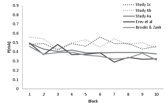
Figure 1: Proportion of choices of the riskier mixed gamble over time
in Study 1c, 4a, 4b, and the studies reported by Erev et al. (2010)
and Brooks and Zank (2005). The data is summarized in 10 blocks of 9
trials. The dashed lines represent studies that included choice
between both similar and different EV prospects (studies 1c, 4b), and
the continuous lines represent studies that focused only on choice
between similar EV prospects (Erev et al., Brooks and Zank, Study 4a).
5.2.1 Experimental Design
Forty two students participated in this study. Each subject was
presented with the 90 choice problems (Appendix 3). Twenty one
subjects were assigned to the mixed condition and 21 to the gain
condition, which was created by the same procedure as in Study 4a. The
order of the problems was randomized for each subject. Subjects
received a show-up fee of 30 Sheqels. At the end of the experiment
one of the problems was randomly selected to determine the subject’s
final payoff, which ranged between 15 and 52 Sheqels ($3.75 and $13,
respectively).
5.2.2 Results and discussion
The right-hand side of Table 7 shows the main results of Study 4b (the
left-hand side shows the results of study 4a). The table reveals that
the overall proportion of risk taking in the mixed condition of Study
4b was 50%. Thus the results show no evidence for absolute loss
aversion. The proportion of risk taking in the gain condition was
significantly lower (26%), t(40) = 4.61, p
< .0001. This result shows a reversed relative loss
aversion tendency, which is in line with the previous study.
The rate of risky choice across the 30 problems with similar EV was
51% in the mixed condition of Study 4b and only 21% in the gain
condition, t(40) = 5.08, p < .0001. Once
again, these observations show no evidence for absolute loss aversion
and significant evidence for reversed relative loss aversion.
An evaluation of the effect of zero payoffs on risk raking in the gain
domain reveals that the proportion of risk taking in the gain domain
was 18% when the low payoff was zero, and 29% when the low payoff
was higher. A paired sample t-test shows that the difference is
significant, t(20) = −3.8, p = .001, suggesting that zero payoffs
from the risky prospect facilitated risk aversion. Yet, even when the
low payoff is larger than zero the level of risk taking was
significantly below 50%, (t(20) = −7.95, p < .0001) and
significantly lower than the risk taking in the mixed domain, t(40) =
4.03, p < .001.
The difference between the results of Study 4a (41% risk taking
between mixed gambles) and Study 4b (50% risk taking between mixed
gambles) suggests that the counter-evidence to absolute loss aversion
is not unique to fifty-fifty prospects. It supports the idea that
simplifying choice, either by focusing on fifty-fifty prospects, or by
increasing the expected value differences even if only in some
problems, may eliminate the tendency to exhibit absolute loss
aversion.
5.3 The effect of repeated experience without feedback, and a speculation
Figure 1 presents the proportion of choices of the riskier mixed
gamble over time in the three long studies presented above (1c, 4a,
and 4b) and in the two published studies that have motivated Study 4a
(Brooks & Zank, 2005; and Erev et al., 2010). The data suggest that
the discrepancy between the different studies increases with time. The
initial behavior in all five studies appear to reflect risk neutrality
(the choice rates in the first block do not differ from 50%), but at
least in some cases experience significantly increase risk aversion.
A paired t-test comparison of risk taking levels per subject between
the first and last block of trials suggests that the increase in risk
aversion with time is significant in the studies that documented an
absolute loss aversion tendency (Study 4a: t(29) = 2.48, p = .019;
Erev et al.: t(39) = 2.17, p = .036, and nearly significant in Brooks
and Zank’s study: t(48) = 1.86, p = .069), but is insignificant in the
other two studies that have not found evidence for loss aversion
(Study 1c: t(21) = 0.32, p = .750; Study 4b: t(20) = 1.44, p = .165).
Recall that the subjects in the current studies did not receive any
feedback concerning the outcomes of their choices. Thus, the effect
of time is not a reflection of reaction to feedback. We speculate
that the effect of time may be an indication of learning without
feedback (Weber, 2003). Specifically, it is possible that at the
initial trials of the experiment the subjects tend to consider several
strategies: compensatory strategies like the expected value
maximization rule or equal weighting (Dawes & Corrigan, 1974), as
well as simpler and non-compensatory strategies like “minimize the
probability of loss” (Payne, 2005; Wu & Markle, 2008) or “maximize
the worst possible payoff”. When all the strategies lead to similar
expected outcomes, the subjects “learn” to favor the simpler
strategies. If the simpler strategies are more likely to imply loss
aversion (e.g., its plausible that taking shortcuts increases
attention to worst case scenarios implied by these shortcuts), the
absolute loss aversion pattern is expected to emerge with time when
these strategies save effort and have little effect on the expected
outcomes (Studies 4a, Erev et al. and Brook & Zank), but not when
the EV maximization rule is easy to use (fifty-fifty studies like 1c)
or when it is easy to see that the simple rules impair expected return
(large REV as in Study 4b).
Partial support for the current speculation is provided by a post-hoc
analysis that focuses on the correlation between the difference
between the prospects’ expected values [EV(safe)-EV(risk)] in the
first block of trials in Study 4b, and the proportion of safe choices
in the subsequent trials. The correlation over the 42 subjects is
positive and significant (r = 0.41, p <
.01). Subjects who experienced that EV(safe) > EV(risky)
in the first block of 9 trials were more likely to prefer the safer
option in subsequent trials (exhibiting an “absolute loss
aversion”), than subjects who experienced EV(safe) <
EV(risky) in the first trials. Thus, early examples of the value of
simple rules that favor the safe option (e.g., “maximize the worst
payoff”) in the first few trials increased the tendency to make
choices consistent with it.
6 Discussion and conclusions
The current paper presents six clarifications of the descriptive value
of the loss aversion assertion in decisions under risk. The first two
clarifications focus on the conditions that give rise to
relative loss aversion (stronger risk aversion in choice
between mixed payoffs that include both gains and losses than in
choice between nonnegative outcomes). The results summarized in Table
4 (Study 1a) show that this tendency emerges when two conditions are
satisfied: (1) the safer prospect increases the probability of
a positive outcome in the mixed domain but not in the gain domain,
and (2) the prospects involve high nominal payoff magnitude. In
addition, Table 4 presents a reversed relative loss aversion tendency
under low nominal payoff magnitude. Our subsequent studies that focus
on low nominal magnitudes (1b, 1c, 3, 4a, and 4b) showed a reversed
relative loss aversion tendency: stronger risk aversion in choice
between gains than between mixed prospects. This pattern was
particularly strong when the safer prospect increases the probability
of a positive outcome in the gain domain (i.e., when the risky
prospect in the gain domain includes a zero outcome) but not in the
mixed domain. Thus, it can be a reflection of a tendency to maximize
the probability of gains (Payne, 2005).
The other clarifications shed light on the conditions that give rise
to absolute loss aversion (risk aversion in choice between
gambles that involve both gains and losses). The most important
clarification in this class involves the effect of framing of
the safe prospect as the status quo: Table 3 (Study 1a) shows that
absolute loss aversion is facilitated by this framing: Absolute loss
aversion appears when people are asked whether they would accept a
gamble (so the gamble is framed as the alternative to the status quo),
and diminishes when people are asked to simply choose between
prospects. Studies 1b and 1c show the robustness of this pattern in
choice among low magnitude fifty-fifty gambles.
A forth clarification involves the magnitude of actual
stakes: Study 2 demonstrates that absolute loss aversion is
observed under high, but not under low stakes.
The fifth clarification involves the use of the choice list paradigm
that facilitates the contrast effect. Study 3 shows a clear
tendency of absolute loss aversion when the risky prospect in the
target problem is relatively unattractive: that is, most of the other
problems include more valuable risky prospects. This tendency was
eliminated when the relative attractiveness of the prospects in the
target problem was balanced.
The final clarification involves the emergence of absolute loss
aversion in long studies with asymmetric gambles. Study 4a shows
evidence for absolute loss aversion in a long study that focuses on
asymmetric gambles with similar expected values. Study 4b shows that
when problems of choice among prospects with significantly different
expected values are also included, the absolute loss aversion tendency
is diminished even in choices between the prospects with similar EV.
We speculate that these and similar results can be captured with the
hypothesis of some learning without feedback. Specifically, it is
possible that the tendency to follow simple strategies that imply loss
aversion increases over time when these strategies are effective
(i.e., when they reduce effort without impairing expected return).
6.1 Two interpretations
The implications of the current results to the loss aversion
hypothesis can be described in two very different ways. One
description implies that each of the six clarifications sheds light on
one manipulation that generates loss aversion, and on the boundaries
of this effect. The alternative description implies that the current
results shed light on manipulations that mask a general loss aversion
tendency.
The “masking” interpretation is consistent with McGraw et al.’s (2010)
demonstration that the judgment of the absolute magnitude losses is
larger than the absolute judgment of gains. However, there are also
important shortcomings of this interpretation. First is the
observation that the judgment results, like the choice results, are
slippery. In a recent paper Yechiam et al. (2013) replicated McGraw
et al.’s findings when the subjects wore eye tracking glasses, and then
eliminated the effect by telling participants that the glasses detect
lies (and that the detection of lies will reduce their payoff).
Yechiam et al. note that this pattern can be a reflection of an
overgeneralization of a complaint bias: People complain (overrate the
losses, and underrate the gains) because there are many situations in
which complaining is effective.
A more significant shortcoming of the “masking” interpretation is
the fact that it is less careful. Unlike the masking interpretation,
the “generators” interpretation describes the current results, and
does not add untested assertions. That is, it does not assume specific
attitude toward losses in the situations that were not studied here.
Another advantage of the generators summary is the observation that at
least five of the current clarifications are reflections of well-known
and robust behavioral tendencies, rather than situation-specific
masks. The effect of nominal (numerical) payoffs on relative loss
aversion can be captured with the assertion that the tendency to
maximize probability of a gain (Payne, 2005) is enhanced by large
nominal (numerical) payoffs. Under one explanation of this pattern it
reflects stronger diminishing sensitivity with the increase of nominal
representation of payoffs (Erev et al., 2008), which seems consistent
with research of the psychophysics of numbers (e.g., Deane, 2007).
The observed sensitivity of absolute loss aversion to the framing of
the safe alternative as the status quo simply reminds us that loss
aversion is only one of many contributors that have been suggested to
explain the status-quo bias (e.g., Anderson, 1993; Gal, 2006; Ritov &
Baron, 1992; Samuelson & Zeckhouser, 1988). Thus, the framing of
option as a status quo increases its attractiveness even when this
framing does not change the predictions of loss aversion as captured
by prospect theory (Kahneman & Tversky, 1979).
Table 8: Empirical estimates of the loss aversion parameter. The described
payoffs are the payoffs described in the experimental task, the actual
payoff is the actual realization of the described payoff (“None”
means that payoffs were hypothetical).
Study
λ estimate
Described payoffs
Actual payoffs
Andersen et al. (2010)
0.78−1.01
Up to $8
−$8 to $8
Reiskamp (2008)
1.00
Up to €100
−€5 to €5
Harrison & Rutström (2009)
1.38
Up to $8
−$8 to $8
Schmidt & Traub (2002)
1.43
Up to DM400
None
Glöckner & Pachur (2011)
1.05−1.99
Up to €1200
€10 to €12
Booij et al. (2010)
1.58
Up to €1000
None
Booij & van de Kuilen (2009)
1.80
Up to €1000
None
Abdellaoui et al. (2007)
2.04
Up to FF40,000
None
Abdellaoui et al. (2008)
2.61
Up to €10,000
0 to €1000*
* One out of 48 subjects was randomly selected and paid only for her choices between gains at rate of 1/10 of the described payoffs.
The effect of payoff magnitude is anything but surprising. As noted
by Rabin (2003) the traditional implementation of expected utility
theory overestimates this effect. Loss aversion is important to
capture risk aversion in choice among low stake gambles, but our
results suggest that this pattern is not general: there are many
situations in which people exhibit risk neutrality in choice among low
stakes mixed gambles.
The large impact of the contrast effect, documented in Study 3, is not
likely to surprise students of the contrast effect. Previous research
has shown the importance of this effect in decisions under risk (see
Stewart et al., 2003). We chose to include a replication of this
well-known effect here because it is often ignored in the study of
loss aversion. We hope that the current clarification of the
significance of this effect will help to reduce this tendency.
Another advantage of the generators summary is implied by the fact
that our research focused on the well-known demonstrations of the loss
aversion pattern (i.e., the Samuelson Colleague’s problem presented in
Table 1 and the Thaler et al. investment problem presented in Table
2). The current results show that each of these demonstrations has
clear boundaries. The evidence for a general loss aversion bias would
look much weaker had we used a different problems selection criterion.
In particular, we could focus on factors that generate behavior that
appears to reflect a reversed loss aversion bias. One example is
betting behavior. The framing of the choice task as a betting game
leads most subjects to participate in betting games with negative
expected return (Sonsino et al., 2002). Another example is
multi-alternative investment decisions with feedback. Ben Zion et
al. (2010) show that in this setting people tend to prefer risky
stocks over safer index funds with higher expected return. A third
example comes from studies of market entry games (Erev, Ert & Roth,
2010). Analysis of the initial behavior in these games shows that
70% of the subjects favor a risky entry to the market that can lead
to unspecified gain or loss, over a safer option. A forth example is
provided by Slovic et al. (2002). They noticed that the addition of
a small loss (of 5 cents) to the gamble “7/36 chance to win $9, and
$0 otherwise” increases the tendency to select it over a safer
prospect with higher expected value. Finally, Yechiam and Hochman
(2013) show that the addition of losses can increase the tendency to
choose a gamble over a safer prospect with lower expected return.
6.2 Quantitative tests
The definitions of the relative and absolute loss aversion, considered
here, are the common qualitative interpretation of loss aversion in
the applications of prospect theory (Camerer, 2000; Thaler et al.,
1997). These interpretations can be derived from prospect theory with
some additional assumptions (concerning the value of the reference
point, the shape of the weighting function, and the concavity of the
value function). Recent studies propose quantitative definitions of
loss aversion, and elegant procedures to estimate this construct (see
theoretical abstractions by Köbberling & Wakker, 2005; Schmidt &
Zank, 2005; Wakker, 2010; Zank, 2008). These procedures allow direct
estimation of the “loss aversion coefficient” (λ ),
controlling for the additional assumptions of prospect theory. This
coefficient captures the tendency to overweight losses; λ = 1
implies equal weighting of gain and losses, and larger values imply
loss aversion.
To clarify the relationship of the current results to this line of
research we present, in Table 8, the estimated loss aversion
coefficient in the studies reviewed by Booij, van Praag, and van de
Kuilen (2010) and two additional recent studies (Glöckner & Pachur,
2011; Reiskamp, 2008). The results reveal large differences between
studies (λ between 0.71 and 2.61) and a strong positive
relationship between the estimated loss aversion parameter (λ
values) and the (described and actual) payoff magnitude. Thus, the
results seem to be consistent with the current analysis; they
demonstrate the contingent nature of loss aversion, and the
significance of two of the contributors to this contingent nature that
were clarified here.
6.3 The adaptive decision maker explanation
The current results are consistent with the adaptive decision maker
idea (Payne, Bettman, & Johnson, 1993; and see related ideas in
Gilboa & Schmeidler, 1995; Gigerenzer & Selten, 2001; and Skinner,
1953). According to this approach decision makers tend to select easy
strategies that have led to the best outcomes in similar cases in the
past. The past experiences that affect behavior in the current
settings can be divided to two classes: Old experiences that occur
before the beginning of the experiment, and new experiences that occur
during the experiment. Study 4b and the data summarized in Figure 1
demonstrate the importance of new experiences: The emergence of
absolute loss aversion in long low-stakes studies can be predicted
based on the cost of using simple rules like the “minimize the
probability of loss”: Absolute loss aversion appear to emerge with
time when such simple rules that implies loss aversion are effective.
That is, minimize effort with a little effect on the expected return.
The other effects, discussed above, can be reflections of
(overgeneralizations from) old experiences. The effect of the
status-quo framing, demonstrated in Tables 1 and 3, can reflect
overgeneralization from past experiences with market for lemons
(Akerlof, 1970). It seems reasonable to assume that the status-quo
framing increase the tendency to rely on past experience with tricky
risky offers like typical SPAM emails (Ert & Erev, 2008).
The effects of the actual and nominal payoff magnitude might reflect
the fact that when the stakes are high it is typically wise to be
careful, and collect as much information as possible. Finally, the
contrast effect might reflect the fact that it is typically wise to
accept the best risky prospect, and avoid the worst risky prospects.
Indeed, relative judgment is the optimal strategy in the many problems
(Freeman, 1983).
6.4 Practical implications
In order to evaluate the practical implications of the contingent
nature of loss aversion, suggested here, we reconsider three of the
best-known natural phenomena that have been explained by loss
aversion. Specifically, we focus on the status-quo bias (Samuelson &
Zeckhauser 1988), the endowment effect (Knetsch & Sinden, 1984;
Thaler, 1980), and underinvestment in stocks (Benartzi & Thaler
1995). The leading explanations of all three phenomena assume a
general loss aversion bias; thus, they appear to be inconsistent with
the contingent interpretation of loss aversion. Yet, two observations
suggest that the existence of these interesting phenomena may actually
emphasize the potential importance of the current results. The first
observation is that loss aversion is only one of many feasible
explanations for these phenomena: Alternative explanations of the
status-quo bias include the omission bias (Baron & Ritov, 1994; Ritov
& Baron, 1992), decision avoidance (Anderson, 2003), and implicit
recommendations (McKenzie, Liersch, & Finkelstein, 2006).
Non-loss-aversion accounts of the endowment effect can be based on
asymmetric information (Dupont & Lee 2002), mere ownership (Brenner
et al. 2007; Morewedge, Shu, Gilbert, & Wilson, 2009),
misconceptions (Plott & Zeiler, 2005) and inertia (Gal, 2006).
Finally, underinvestment in stocks can the explained without loss
aversion by assuming monetary constraints (Constantinides, Donaldson,
& Mehra, 2010), habit persistence (Constantinides, 1990), impact of
rare disastrous events (Rietz, 1988) and/or incomplete markets
(Aiyagari & Gertler, 1991).
A second, and more important, observation concerns the generality of
the trend suggested by the phenomena explained by loss aversion. It
is easy to find natural phenomena that appear to reflect reversals of
the phenomena that were explained by “loss aversion”. One example is
“overtrading in the stock market” (Odean, 1999). The term
“overtrading” captures the fact that people tend to trade more than
predicted under the rational model; overtrading appears to reflect a
reversal of the status-quo bias. Thus, under the assumption that the
status-quo bias reflects loss aversion, overtrading might be described
as a reflection of a reversed loss aversion bias. A second example is
overbidding in auctions (see a recent review by Kagel & Levin, in
press) that might reflect a reversal of the endowment effect. The
endowment effect implies that potential buyers undervalue products
that they do not own, while overbidding could imply the opposite.
Finally, analyses of investments decisions reflect “insufficient
diversification” (Barber & Odean, 2000; Ben Zion, Erev, Haruvy, &
Shavit, 2010; Polkovnichenko, 2005) that could imply risk seeking.
Thus, if risk aversion in the stock market reflects loss aversion
(Benarzi & Thaler, 1995), insufficient diversification can be
described as a reversed loss aversion bias.
In other words, the current results suggest that the contingent nature
of loss aversion should be considered in the analysis of field data.
Whereas most previous attempts to relate the loss aversion assertion
to field research focused on phenomena that can be explained as
reflections of loss aversion, it is easy to think of phenomena that
can be explained with the opposite bias. Namely, it is possible that
better understanding of the contingent nature of loss aversion can be
of practical value.
6.5 Summary
Most applications of loss aversion interpreted it to mean that people
exhibit stronger risk aversion in choices that involve possible gains
and losses than in choices that involve only gains. The current
results reject this assertion; they show weaker risk aversion in
choice between mixed prospects than in choice between gains.
Moreover, in a wide set of conditions, decisions among mixed prospects
show a choice pattern that is more consistent with risk neutrality
than with risk aversion. These results can be captured with the
assertion that the exact effect of losses does not result from a
stable perceptual construct: losses do not always loom larger than
gains. Rather, the results highlight six specific conditions that
trigger the pattern predicted by the loss aversion assertion.
References
Abdellaoui, M., Bleichrodt, H., & Paraschiv, C. (2007). Loss aversion
under Prospect theory: A parameter free
measurement. Management Science, 53, 1659–1674.
Abdellaoui, M., Bleichrodt, H., & Haridon, O. L. (2008). A tractable
method to measure utility and loss aversion under prospect
theory. Journal of Risk and Uncertainty, 36,
245–266.
Aiyagari, S. R., & Gertler, M. (1991). Asset returns with
transactions costs and uninsured individual risk. Journal of
Monetary Economics, 27, 311–331.
Akerlof, G. A. (1970). The market for “lemons”: Quality uncertainty
and the market mechanism. The Quarterly Journal of Economics,
84, 488–500.
Andersen, S., Harrison, G.W., Lau,M. I., & Rutström,
E. E. (2010). Behavioral econometrics for psychologists.
Journal of Economic Psychology, 31, 553–576.
Anderson, C. J. (2003). The psychology of doing nothing: Forms of
decision avoidance result from reason and emotion.
Psychological Bulletin, 129, 139–167.
Barber, B. M., & Odean, T. (2000). Trading is hazardous to your
wealth: The common stock investment performance of individual
investors. The Journal of Finance, 55, 773–806.
Baron, J., & Ritov, I. (1994). Reference points and omission
bias. Organizational Behavior and Human Decision Processes,
59, 475–498.
Barron, G., & Erev, I. (2003). Small feedback-based decisions and their
limited correspondence to description-based decisions. Journal of
Behavioral Decision Making, 16, 215–233.
Battalio, R., Kagel, J., & Jiranyakul, K. (1990). Testing between
alternative models of choice under uncertainty: Some initial
results. Journal of Risk and Uncertainty, 3, 25-50.
Benartzi, S., & Thaler, R. H. (1995). Myopic loss aversion and the
equity premium puzzle. The Quarterly Journal of Economics,
110, 73–92.
Ben Zion, U., Erev, I., Haruvy, E., & Shavit, T. (2010). Adaptive
behavior leads to under-diversification. Journal of Economic
Psychology, 31, 985–995.
Booij, A. S., & van de Kuilen, G. (2009). A parameter-free analysis
of the utility of money for the general population under prospect
theory. Journal of Economic Psychology, 30,
651–666.
Booij, A. S., van Praag, B. & van de Kuilen, G. (2010). A parametric
analysis of prospect theory’s functionals for the general
population. Theory and Decision, 68, 115–148.
Brenner, L., Rottenstreich, Y., Sood S., & Bilgin, B. (2007). On the
psychology of loss aversion: Possession, valence, and reversals of the
endowment effect. Journal of Consumer Research, 34,
369–376.
Brooks, P., & Zank, H. (2005). Loss averse behavior. Journal
of Risk and Uncertainty, 31, 301–325.
Camerer, C. (2000). Prospect theory in the wild: Evidence from the
field. In C. Camerer, G. Loewenstein, & M. Rabin (Eds),
Advances in behavioral economics, pp. 148–161. New York:
Princeton University Press.
Constantinides, G. M. (1990). Habit formation: A resolution of the
equity premium puzzle. The Journal of Political Economy,
98, 519–543.
Constantinides, G. M., Donaldson, J. B., & Mehra, R. (2010). Junior
can’t borrow: A new perspective on the equity premium
puzzle. Quarterly Journal of Economics, 117,
269–296.
Coombs, C. H., & Pruitt, D. G. (1960). Components of risk in decision
making: Probability and variance preferences. Journal of
Experimental Psychology, 60, 265.
Dawes, R. M., & Corrigan, B. (1974). Linear models in decision
making. Psychological Bulletin, 81, 95-106.
Dehaene, S. (2007). Symbols and quantities in parietal cortex:
Elements of a mathematical theory of number representation and
manipulation. In P. Haggard, Y. Rosseti, & M. Kawato (Eds.),
Attention & performance XXII. Sensori-motor foundations of
higher cognition, pp. 527–574. Cambridge, MA: Harvard University Press.
Dupont, D. Y., & Lee, G. S. (2002). The endowment effect, status-quo
bias and loss aversion: Rational alternative
explanation. Journal of Risk and Uncertainty, 25,
87–101.
Erev, I., Ert, E., Roth, A., Haruvy, E., Herzog, S., Hau, R., Hertwig,
R., Stewart, T., West, R., & Lebiere, C. (2010). A choice prediction
competition for choices from experience and from
description. Journal of Behavioral Decision Making,
23, 15–47.
Erev, I., Ert, E., & Roth, A. E. (2010). A choice prediction
competition for market entry games: An introduction. Games,
1, 117–136.
Erev, I., Ert, E., & Yechiam, E. (2008). Loss aversion, diminishing
sensitivity, and the effect of experience on repeated
decisions. Journal of Behavioral Decision Making,
21, 575–597.
Ert, E., & Erev, I. (2008). The rejection of attractive gambles, loss
aversion, and the lemon avoidance heuristic. Journal of
Economic Psychology, 29, 715–723.
Fehr, E., & Goette, L. (2007). Do workers work more if wages are
high? Evidence from a randomized field experiment. The
American Economic Review, 97, 298–317.
Freeman, P. R. (1983). The secretary problem and its extensions: A
review. International Statistical Review, 51, 189–206.
Gaechter, S., Johnson, E., & Herrmann, A. (2010). Individual-level
loss aversion in riskless and risky choices.
http://econpapers.repec.org/paper/cdxdpaper/2010-20.htm
Gal, D. (2006). A psychological law of inertia and the illusion of
loss aversion. Judgment and Decision Making, 1,
23–32.
Gigerenzer, G., & Selten, R. (2001). Bounded rationality: The
adaptive toolbox. Cambridge, MA: MIT Press.
Gilboa, I., & Schmeidler, D. (1995). Case-based decision
theory. The Quarterly Journal of Economics, 110,
605–639.
Glöckner, A., & Pachur, T. (2012). Cognitive models of risky
choice: Parameter stability and predictive accuracy of prospect
theory. Cognition, 123, 21–32.
Harrison, G. W., & Rutström, E. E. (2009). Expected utility theory
and prospect theory: One wedding and a decent
funeral. Experimental Economics, 12,133–158.
Harinck, F., Van Dijk, E., Van Beest, I., & Mersmann, P. (2007). When
gains loom larger than losses: Reversed loss aversion for small
amounts of money. Psychological Science, 18,
1099–1105.
Holt, C. A., & Laury, S. K. (2002). Risk aversion and incentive
effects. The American Economic Review, 92,
1644–1655.
Kagel, J. H., & Levin, D. (in press). Auctions: A survey of
experimental research, 1995–2008. In Roth, A. & Kagel, J.
eds. The Handbook of Experimental Economics (Vol. 2).
Kahneman, D., & Tversky, A. (1979). Prospect Theory: An analysis of
decision under risk. Econometrica, 47, 263–291.
Knetsch, J. L., & Sinden, J. A. (1984). Willingness to pay and
compensation demanded: Experimental evidence of an unexpected
disparity in measures of value. The Quarterly Journal of
Economics, 99, 507–521.
Köbberling, V., & Wakker, P. P. (2005). An index of loss
aversion. Journal of Economic Theory, 122, 119-131.
McGraw, A. P., Larsen, J. T., Kahneman, D., & Schkade,
D. (2010). Comparing gains and losses. Psychological science,
21, 1438–1445.
McKenzie, C. R. M., Liersch, M. J., & Finkelstein,
S. R. (2006). Recommendations implicit in policy defaults.
Psychological Science, 17, 414 -420.
Morewedge, C. K., Shu, L. L., Gilbert, D. T., & Wilson,
T. D. (2009). Bad riddance or good rubbish? Ownership and not loss
aversion causes the endowment effect. Journal of Experimental
Social Psychology, 45, 947–951.
Novemsky, N., & Kahneman, D. (2005). The boundaries of loss
aversion. Journal of Marketing Research, 42,
119–128.
Odean, T. (1999). Do investors trade too much? American
Economic Review, 89, 1279–1298.
Pandelaere, M., Briers, B., & Lembregts, C. (2011). How to make a
29% increase look bigger: The unit effect in option
comparisons. Journal of Consumer Research, 38,
308–322.
Payne, J. W. (2005). It is whether you win or lose: The importance of
the overall probabilities of winning or losing in risky
choice. Journal of Risk and Uncertainty, 30, 5–19.
Payne, J. W., Bettman, J. R., & Johnson, E. J. (1993). The
adaptive decision maker. Cambridge, England: Cambridge University
Press.
Plott, C. R., & Zeiler, K. (2005). The willingness to pay-willingness
to accept gap, the “endowment effect,” subject misconceptions, and
experimental procedures for eliciting valuations. The American
Economic Review, 95, 530–545.
Polkovnichenko, V. (2005). Household portfolio diversification: A case
for rank-dependent preferences. Review of Financial Studies,
18, 1467 -1502.
Rabin, M. (2003). Risk aversion and expected-utility theory: A
calibration theorem. Econometrica, 68, 1281–1292.
Raghubir, P. & Srivastava, J. (2002). Effect of face value on product
valuation in foreign currencies. Journal of Consumer
Research, 29, 335–347.
Redelmeier, D. A., & Tversky, A. (1992). On the framing of multiple
prospects. Psychological Science, 3, 191 -193.
Rieskamp, J. (2008). The probabilistic nature of preferential
choice. Journal of Experimental Psychology: Learning, Memory,
and Cognition, 34, 1446–1465.
Rietz, T. A. (1988). The equity risk premium a
solution. Journal of Monetary Economics, 22,
117–131.
Ritov, I., & Baron, J. (1992). Status-quo and omission
biases. Journal of Risk and Uncertainty, 5, 49-61.
Rottenstreich, Y., Burson, K., & Faro, D. (2013). Multiple unit
holdings yield attenuated endowment effect. Management
Science, 59, 545-555.
Samuelson, P. A. (1963). Risk and uncertainty: A fallacy of large
numbers. Scientia, 98, 108–113.
Samuelson, W., & Zeckhauser, R. (1988). Status quo bias in decision
making. Journal of Risk and Uncertainty, 1, 7–59.
Schmidt, U., S. Traub. (2002). An experimental test of loss
aversion. Journal of Risk and Uncertainty, 25,
233–249.
Schmidt, U., & Zank, H. (2005). What is loss aversion?
Journal of Risk and Uncertainty, 30, 157–167.
Sherif, M., Taub, D., & Hovland, C. I. (1958). Assimilation and contrast
effects of anchoring stimuli on judgments. Journal of Experimental
Psychology, 55, 150–155.
Sherif, M., & Hovland, C. I. (1961). Social judgment. New Haven: Yale
University Press.
Skinner, B.F. (1953). Science and Human Behavior. New York:
Free Press.
Sonsino, D., Erev, I., & Gilat, S. (2002). On rationality,
learning and zero-sum betting—an experimental study of the
no-betting conjecture. Mimeo, Technion University.
Stewart, N., Chater, N., Stott, H. P., & Reimers, S. (2003). Prospect
relativity: How choice options influence decisions under
risk. Journal of Experimental Psychology: General,
132, 23–46.
Schwarz, N. (1999). Self-reports: How the questions shape the
answers. American Psychologist, 54, 93–105.
Slovic, P., Finucane, M. L., Peters, E., & MacGregor,
D. G. (2002). The affect heuristic. In T. Gilovich, D. Griffin, &
D. Kahneman, Eds., Heuristics and biases: The psychology of
intuitive judgment, pp. 397–420. New York: Cambridge University
Press.
Thaler, R. (1980). Toward a positive theory of consumer
choice. Journal of Economic Behavior & Organization, 1,
39–60.
Thaler, R. H., & Johnson, E. J. (1990). Gambling with the house money
and trying to break even: The effects of prior outcomes on risky
choice. Management Science, 36, 643–660.
Thaler, R. H., Tversky, A., Kahneman, D., & Schwartz, A. (1997). The
effect of myopia and loss aversion on risk taking: An experimental
test. Quarterly Journal of Economics, 112, 647–661.
Tversky, A., & Kahneman, D. (1992). Advances in prospect theory:
Cumulative representation of uncertainty. Journal of Risk and
Uncertainty, 5, 297–323.
Wakker, P. P. (2010). Prospect theory: For risk and
ambiguity. Cambridge University Press.
Wakker, P. P. (2013). Annotated references on decisions and
uncertainty. Websource downloaded on March 27, 2013, from
http://people.few.eur.nl/wakker/
Weber, R. A. (2003). ’Learning’ with no feedback in a competitive
guessing game. Games and Economic Behavior, 44,
134–144.
Weber, B. J. & Chapman, G. B. (2005). Playing for peanuts: why is
risk seeking more common for low-stakes gambles?
Organizational Behavior & Human Decision Processes, 97,
31–46.
Wu, G., & Markle, A. B. (2008). An empirical test of gain-loss
separability in prospect theory. Management Science,
54, 1322–1335.
Yechiam, E., & Ert, E. (2011). Risk attitude in decision making: In
search of trait-like constructs. Topics in Cognitive Science,
3, 166–186.
Yechiam, E., & Hochman, G. (2013). Loss-aversion or loss-attention:
The impact of losses on cognitive performance. Cognitive
Psychology, 66, 212-231.
Yechiam, E., Telpaz, A., & Hochman, G. (2013). The complaint bias in
subjective evaluations of incentives. Manuscript, Technion University.
Zank, H. (2008). On probabilities and loss aversion. Theory
and Decision, 68, 243–261.
Appendix 1. The 90 mixed problems evaluated in study 1c.
Prob.
S1
Ps
S2
R1
Pr
R2
Pr-mix
Pr-gain
Prob.
S1
Ps
S2
R1
Pr
R2
Pr-mix
Pr-gain
1
7
0.5
−8
11
0.5
−11
0.77
0.50
46
7
0.5
−7
9
0.5
−9
0.45
0.58
2
6
0.5
−6
13
0.5
−16
0.00
0.38
47
5
0.5
−5
8
0.5
−8
0.50
0.38
3*
12
0.5
−12
11
0.5
−14
0.09
0.17
48
9
0.5
−9
12
0.5
−12
0.41
0.25
4
4
0.5
−6
13
0.5
−13
0.73
0.33
49
6
0.5
−6
10
0.5
−10
0.59
0.29
5
11
0.5
−11
12
0.5
−13
0.05
0.21
50
4
0.5
−4
11
0.5
−11
0.50
0.33
6
7
0.5
−7
9
0.5
−10
0.14
0.42
51
5
0.5
−5
12
0.5
−11
0.64
0.29
7
4
0.5
−4
9
0.5
−12
0.09
0.21
52
4
0.5
−4
7
0.5
−6
0.68
0.33
8
5
0.5
−5
7
0.5
−8
0.05
0.46
53
11
0.5
−9
12
0.5
−11
0.27
0.29
9
5
0.5
−5
12
0.5
−14
0.00
0.17
54
5
0.5
−2
6
0.5
−6
0.05
0.25
10
7
0.5
−7
8
0.5
−11
0.05
0.29
55
8
0.5
−5
13
0.5
−13
0.18
0.29
11
9
0.5
−9
11
0.5
−12
0.18
0.33
56
10
0.5
−10
13
0.5
−12
0.64
0.54
12*
10
0.5
−13
12
0.5
−12
0.91
0.75
57
8
0.5
−7
11
0.5
−11
0.32
0.50
13
5
0.5
−6
9
0.5
−9
0.77
0.42
58
12
0.5
−9
13
0.5
−13
0.18
0.21
14
8
0.5
−8
12
0.5
−15
0.18
0.21
59*
7
0.5
−5
6
0.5
−6
0.05
0.13
15
9
0.5
−10
11
0.5
−11
0.82
0.75
60
6
0.5
−6
12
0.5
−11
0.59
0.50
16
5
0.5
−8
13
0.5
−13
0.73
0.67
61
4
0.5
−4
6
0.5
−5
0.91
0.92
17
7
0.5
−7
10
0.5
−11
0.09
0.21
62
6
0.5
−6
10
0.5
−9
0.68
0.46
18
8
0.5
−9
10
0.5
−10
0.86
0.75
63
6
0.5
−3
8
0.5
−8
0.14
0.17
19
10
0.5
−10
12
0.5
−14
0.05
0.21
64
4
0.5
−1
5
0.5
−5
0.00
0.29
20
11
0.5
−11
14
0.5
−13
0.73
0.54
65
8
0.5
−8
12
0.5
−9
0.86
0.79
21
4
0.5
−4
6
0.5
−7
0.05
0.38
66
8
0.5
−6
12
0.5
−12
0.27
0.13
22
9
0.5
−9
11
0.5
−10
0.86
0.63
67
5
0.5
−5
12
0.5
−10
0.73
0.58
23
11
0.5
−11
13
0.5
−12
0.91
0.63
68
6
0.5
−6
13
0.5
−11
0.59
0.54
24
6
0.5
−9
12
0.5
−12
0.73
0.63
69
6
0.5
−6
11
0.5
−9
0.77
0.71
25
7
0.5
−7
8
0.5
−11
0.05
0.17
70
8
0.5
−8
11
0.5
−10
0.59
0.63
26
6
0.5
−8
11
0.5
−11
0.82
0.46
71
11
0.5
−8
12
0.5
−12
0.09
0.33
27
11
0.5
−11
12
0.5
−13
0.14
0.42
72
10
0.5
−10
13
0.5
−11
0.82
0.58
28
5
0.5
−6
11
0.5
−11
0.64
0.46
73
8
0.5
−8
10
0.5
−9
0.86
0.58
29
5
0.5
−7
8
0.5
−8
0.91
0.75
74
7
0.5
−6
8
0.5
−8
0.27
0.38
30
4
0.5
−4
5
0.5
−6
0.14
0.21
75
6
0.5
−4
10
0.5
−10
0.18
0.38
31
6
0.5
−7
12
0.5
−12
0.77
0.33
76
11
0.5
−10
13
0.5
−13
0.27
0.21
32
10
0.5
−10
11
0.5
−12
0.05
0.29
77
4
0.5
−3
5
0.5
−5
0.23
0.21
33
6
0.5
−6
7
0.5
−8
0.05
0.25
78
5
0.5
−5
10
0.5
−8
0.68
0.46
34
9
0.5
−9
13
0.5
−14
0.18
0.13
79
9
0.5
−9
11
0.5
−10
0.86
0.54
35
4
0.5
−6
9
0.5
−9
0.82
0.54
80
9
0.5
−9
12
0.5
−10
0.82
0.67
36
4
0.5
−5
9
0.5
−9
0.86
0.58
81
6
0.5
−6
9
0.5
−7
0.86
0.83
37
6
0.5
−6
8
0.5
−9
0.09
0.29
82
9
0.5
−9
11
0.5
−10
0.73
0.83
38
4
0.5
−7
13
0.5
−13
0.86
0.33
83
7
0.5
−6
13
0.5
−13
0.23
0.46
39
2
0.5
−3
9
0.5
−9
0.68
0.38
84
8
0.5
−8
12
0.5
−10
0.68
0.46
40
4
0.5
−4
6
0.5
−7
0.05
0.21
85
7
0.5
−7
10
0.5
−8
0.86
0.75
41
5
0.5
−5
11
0.5
−11
0.45
0.42
86
5
0.5
−5
11
0.5
−10
0.68
0.42
42
1
0.5
−1
10
0.5
−10
0.45
0.38
87
5
0.5
−5
10
0.5
−7
0.86
0.54
43
5
0.5
−5
6
0.5
−6
0.73
0.67
88
4
0.5
−3
8
0.5
−8
0.18
0.25
44
4
0.5
−4
5
0.5
−5
0.55
0.33
89
4
0.5
−4
7
0.5
−5
0.91
0.46
45
4
0.5
−4
7
0.5
−7
0.50
0.50
90
9
0.5
−8
10
0.5
−10
0.32
0.42
Proportion of risk taking across problems without dominant strategy: Mixed: 0.48, Gain: 0.43
Note: Each problem involved a choice between a safer prospect (S1, Ps; S2) and a riskier
(higher variability, or in the case of equal variability: larger
losses) prospect (R1, Pr; R2).The columns Pr-mix and Pr-gain present
the proportion of choices in the riskier prospect (R) in each of
those problems in the mixed and gain conditions respectively (*in
three problems one of the prospects dominates the other: the safer
prospect is the dominant choice in Problems 3 and 59, and the risky
prospect is the dominant choice in Problem 12).
Appendix 2. The 90 mixed problems evaluated in study 4a.
Prob.
S1
Ps
S2
R1
Pr
R2
Pr-mix
Pr-gain
Prob.
S1
Ps
S2
R1
Pr
R2
Pr-mix
Pr-gain
1
7
0.38
−6
16
0.47
−16
0.57
0.20
46
8
0.46
−9
15
0.46
−15
0.40
0.27
2
9
0.57
−2
10
0.8
−18
0.37
0.27
47
3
0.51
−8
11
0.46
−14
0.37
0.20
3
10
0.49
−7
16
0.54
−16
0.43
0.23
48
6
0.52
−7
12
0.55
−15
0.50
0.33
4
10
0.5
−4
13
0.57
−10
0.50
0.20
49
10
0.46
−5
19
0.51
−16
0.50
0.27
5
8
0.5
−10
11
0.45
−11
0.53
0.57
50
7
0.49
−10
16
0.37
−12
0.23
0.30
6
8
0.51
−3
14
0.64
−18
0.50
0.17
51
10
0.39
−1
14
0.59
−12
0.40
0.23
7
1
0.57
−6
15
0.5
−19
0.30
0.17
52
6
0.55
−3
17
0.58
−19
0.43
0.20
8
4
0.47
−2
13
0.57
−15
0.43
0.23
53
9
0.52
−3
11
0.66
−12
0.57
0.40
9
8
0.53
−9
17
0.39
−11
0.30
0.43
54
9
0.47
−6
13
0.61
−18
0.63
0.23
10
3
0.38
−10
10
0.44
−17
0.77
0.20
55
4
0.54
−5
19
0.4
−13
0.20
0.07
11
11
0.36
−11
15
0.4
−15
0.60
0.20
56
2
0.54
−3
16
0.52
−18
0.30
0.13
12
11
0.41
−10
18
0.33
−11
0.37
0.40
57
10
0.53
−9
17
0.45
−12
0.40
0.23
13
4
0.37
−8
18
0.37
−16
0.40
0.37
58
1
0.56
−9
17
0.24
−10
0.43
0.33
14
8
0.57
−7
18
0.54
−18
0.23
0.27
59
4
0.59
−5
17
0.44
−13
0.23
0.07
15
10
0.37
−6
14
0.51
−15
0.57
0.43
60
11
0.36
−5
15
0.43
−10
0.57
0.23
16
7
0.36
−4
14
0.55
−17
0.40
0.27
61
7
0.36
−4
19
0.47
−17
0.53
0.30
17
3
0.62
−4
14
0.56
−17
0.33
0.17
62
11
0.49
−2
16
0.64
−16
0.37
0.37
18
8
0.56
−5
18
0.54
−16
0.17
0.13
63
1
0.5
−1
14
0.44
−11
0.40
0.47
19
8
0.4
−2
14
0.56
−13
0.53
0.50
64
4
0.38
−6
15
0.43
−15
0.50
0.23
20
6
0.55
−5
12
0.5
−10
0.20
0.23
65
6
0.42
−10
13
0.47
−18
0.50
0.13
21
3
0.65
−5
11
0.6
−16
0.23
0.30
66
7
0.39
−10
12
0.33
−11
0.53
0.47
22
6
0.59
−6
16
0.56
−18
0.20
0.27
67
11
0.57
−6
17
0.6
−16
0.33
0.30
23
6
0.4
−10
12
0.42
−15
0.73
0.63
68
6
0.38
−4
17
0.43
−13
0.57
0.23
24
10
0.63
−2
13
0.7
−12
0.20
0.20
69
6
0.57
−11
18
0.36
−12
0.27
0.27
25
7
0.4
−11
15
0.41
−17
0.43
0.37
70
2
0.4
−4
14
0.44
−14
0.43
0.37
26
3
0.45
−7
18
0.29
−11
0.20
0.23
71
6
0.41
−10
15
0.34
−13
0.43
0.40
27
4
0.47
−6
15
0.44
−14
0.27
0.20
72
11
0.57
−11
19
0.54
−19
0.10
0.30
28
9
0.5
−2
16
0.57
−13
0.40
0.37
73
8
0.46
−4
14
0.62
−19
0.57
0.37
29
7
0.67
−10
18
0.53
−17
0.23
0.10
74
7
0.56
−8
13
0.52
−13
0.43
0.23
30
2
0.41
−10
17
0.31
−15
0.47
0.30
75
7
0.65
−11
12
0.64
−19
0.27
0.30
31
9
0.66
−9
11
0.66
−13
0.47
0.30
76
2
0.65
−10
17
0.42
−16
0.37
0.30
32
2
0.6
−10
13
0.49
−18
0.43
0.20
77
4
0.36
−9
17
0.24
−11
0.47
0.47
33
2
0.45
−6
16
0.41
−15
0.47
0.20
78
3
0.58
−6
16
0.51
−18
0.43
0.10
34
9
0.41
−4
19
0.46
−14
0.43
0.20
79
6
0.41
−5
17
0.42
−13
0.40
0.27
35
10
0.42
−10
13
0.39
−11
0.43
0.33
80
6
0.34
−5
11
0.55
−16
0.53
0.27
36
8
0.43
−8
18
0.44
−16
0.47
0.20
81
4
0.47
−8
15
0.47
−18
0.40
0.23
37
8
0.65
−1
14
0.65
−12
0.13
0.03
82
8
0.5
−7
14
0.56
−17
0.47
0.33
38
9
0.61
−5
14
0.58
−11
0.30
0.20
83
7
0.64
−10
15
0.46
−11
0.27
0.30
39
4
0.65
−3
17
0.43
−10
0.27
0.30
84
11
0.61
−1
12
0.81
−18
0.57
0.43
40
1
0.63
−9
14
0.44
−16
0.40
0.20
85
4
0.51
−9
18
0.4
−16
0.23
0.10
41
1
0.49
−8
16
0.35
−14
0.30
0.33
86
3
0.47
−3
19
0.34
−10
0.20
0.30
42
5
0.54
−10
11
0.41
−11
0.47
0.47
87
2
0.5
−7
14
0.47
−17
0.53
0.20
43
6
0.37
−4
12
0.47
−11
0.50
0.23
88
9
0.6
−8
12
0.67
−18
0.57
0.40
44
5
0.56
−7
14
0.45
−12
0.33
0.43
89
9
0.6
−9
10
0.71
−18
0.63
0.60
45
11
0.55
−8
14
0.59
−14
0.63
0.10
90
3
0.55
−8
14
0.49
−17
0.33
0.23
Mean P(risk) across problems: Mixed: 0.41, Gain: 0.28
Note: The notations are the same as in Appendix 1.
Appendix 3. The 90 mixed problems evaluated in study 4b.
Prob.
S1
Ps
S2
R1
Pr
R2
Pr-mix
Pr-gain
Prob.
S1
Ps
S2
R1
Pr
R2
Pr-mix
Pr-gain
1
4
0.52
−10
7
0.49
−16
0.05
0.10
46
10
0.48
−4
16
0.51
−7
0.81
0.38
2
5
0.54
−4
10
0.49
−12
0.33
0.05
47
4
0.46
−5
12
0.51
−10
0.71
0.62
3
3
0.52
−9
7
0.47
−15
0.29
0.05
48
9
0.48
−3
15
0.53
−7
0.86
0.43
4
4
0.57
−3
6
0.5
−8
0.14
0.00
49
3
0.43
−4
8
0.5
−6
0.86
0.52
5
5
0.63
−5
6
0.67
−14
0.33
0.00
50
5
0.37
−5
14
0.33
−6
0.86
0.52
6
7
0.56
−5
10
0.49
−10
0.14
0.00
51
5
0.44
−7
10
0.51
−10
0.71
0.48
7
3
0.58
−9
7
0.5
−15
0.29
0.05
52
9
0.42
−3
15
0.5
−7
0.67
0.19
8
7
0.42
−6
11
0.41
−12
0.29
0.05
53
6
0.58
−7
12
0.59
−11
0.67
0.43
9
4
0.42
−6
6
0.42
−11
0.29
0.05
54
6
0.58
−4
11
0.58
−6
0.90
0.76
10
3
0.39
−5
4
0.47
−11
0.19
0.00
55
5
0.61
−3
11
0.53
−4
0.71
0.71
11
1
0.38
−9
4
0.49
−18
0.52
0.19
56
9
0.62
−1
18
0.51
−4
0.38
0.38
12
11
0.64
−9
13
0.6
−15
0.14
0.05
57
9
0.36
−11
15
0.4
−13
0.67
0.62
13
9
0.42
−4
10
0.47
−10
0.29
0.00
58
4
0.58
−9
10
0.53
−10
0.81
0.62
14
7
0.55
−10
10
0.51
−16
0.24
0.05
59
10
0.45
−7
16
0.49
−10
0.71
0.57
15
8
0.46
−10
10
0.49
−17
0.29
0.10
60
10
0.54
−8
17
0.51
−10
0.62
0.62
16
5
0.65
−7
9
0.64
−14
0.52
0.10
61
7
0.35
−5
14
0.36
−9
0.71
0.14
17
3
0.47
−5
8
0.46
−9
0.62
0.24
62
5
0.53
−3
9
0.54
−8
0.38
0.05
18
10
0.53
−10
14
0.5
−13
0.38
0.05
63
10
0.47
−10
13
0.5
−14
0.52
0.14
19
3
0.58
−7
7
0.57
−12
0.43
0.10
64
7
0.42
−3
12
0.43
−7
0.52
0.29
20
10
0.54
−11
16
0.49
−15
0.33
0.24
65
11
0.46
−10
15
0.51
−16
0.67
0.24
21
6
0.4
−3
9
0.53
−9
0.76
0.33
66
3
0.6
−6
9
0.47
−9
0.33
0.52
22
2
0.66
−9
6
0.63
−15
0.57
0.10
67
9
0.34
−2
15
0.37
−6
0.57
0.38
23
3
0.58
−8
6
0.62
−14
0.57
0.29
68
8
0.42
−3
14
0.38
−6
0.62
0.29
24
3
0.59
−4
8
0.48
−7
0.33
0.14
69
4
0.41
−3
7
0.52
−8
0.71
0.10
25
2
0.65
−6
7
0.59
−12
0.67
0.10
70
6
0.35
−2
12
0.41
−7
0.52
0.29
26
10
0.46
−7
13
0.53
−13
0.57
0.14
71
7
0.54
−10
13
0.47
−13
0.38
0.29
27
8
0.56
−10
11
0.6
−16
0.48
0.00
72
10
0.44
−8
16
0.4
−11
0.43
0.29
28
1
0.37
−5
4
0.58
−12
0.57
0.43
73
5
0.63
−1
12
0.42
−4
0.24
0.29
29
10
0.43
−5
14
0.5
−11
0.38
0.19
74
5
0.57
−10
11
0.5
−14
0.57
0.33
30
6
0.67
−8
10
0.59
−11
0.52
0.10
75
8
0.33
−6
11
0.41
−10
0.52
0.10
31
9
0.65
−5
15
0.61
−8
0.76
0.76
76
5
0.35
−9
8
0.39
−15
0.14
0.14
32
2
0.64
−3
10
0.57
−8
0.71
0.38
77
3
0.36
−2
8
0.43
−10
0.43
0.10
33
2
0.49
−6
8
0.52
−9
0.81
0.62
78
6
0.51
−2
9
0.48
−8
0.14
0.00
34
9
0.36
−9
16
0.39
−11
0.86
0.62
79
9
0.64
−9
11
0.61
−16
0.19
0.00
35
7
0.45
−10
12
0.53
−14
0.81
0.38
80
10
0.55
−7
14
0.47
−12
0.19
0.05
36
7
0.62
−6
14
0.55
−8
0.52
0.33
81
6
0.38
−7
8
0.45
−14
0.24
0.05
37
11
0.66
−2
18
0.57
−4
0.48
0.67
82
2
0.34
−11
4
0.43
−18
0.52
0.14
38
1
0.36
−9
10
0.39
−12
0.76
0.48
83
9
0.64
−1
12
0.61
−10
0.05
0.05
39
6
0.46
−6
13
0.48
−9
0.62
0.57
84
6
0.54
−6
9
0.52
−13
0.29
0.00
40
2
0.46
−7
8
0.51
−10
0.90
0.71
85
7
0.54
−2
10
0.49
−8
0.14
0.05
41
7
0.37
−4
15
0.38
−6
0.71
0.62
86
4
0.63
−7
6
0.62
−15
0.29
0.10
42
8
0.66
−6
15
0.59
−9
0.67
0.48
87
6
0.34
−8
9
0.41
−15
0.29
0.05
43
1
0.43
−5
9
0.37
−6
0.76
0.43
88
5
0.57
−1
6
0.63
−9
0.24
0.05
44
3
0.63
−8
8
0.65
−12
0.81
0.48
89
8
0.37
−3
12
0.35
−8
0.33
0.14
45
4
0.37
−3
11
0.48
−7
0.76
0.29
90
3
0.63
−4
7
0.52
−11
0.19
0.10
Mean P(risk) across problems: Mixed: 0.50, Gain: 0.26
Note: The notations are the same as in Appendix 1.
Dept. of Agricultural Economics
and Management, Faculty of Agriculture, Food, and Environment, The
Hebrew University of Jerusalem, Rehovot 76100,
Israel. Email: eyal.ert@mail.huji.ac.il.
Studies from other research domains
confirm that people seem to be mainly influenced by nominal rather
than actual values. This tendency affects spending behavior when
using foreign currencies (Raghubir & Srivastava, 2002), and lead to
higher perceived difference between attributes when they are
expressed in larger scales, e.g., 900/1000 vs. 800/1000 as opposed
to 9/10 vs. 8/10, (Pandelaere, Briers, & Lembregts, 2011).
After applying this criterion we were left with 63 and 59 subjects
in the high and low magnitude conditions respectively. Including
all 150 subjects in the analysis does not change the main results.
This prediction of
prospect theory was supported by many previous studies. For
example, only 35% of the subjects in Erev et al.’s (2010) decisions
from description condition preferred the gamble “11.5 with
probability 0.6; 3.7 otherwise” (expected value of 8.08) over a
sure gain of 7.9.
We also checked for possible order effects: neither
the ordering of the two problems, nor the ordering of the two
experiments had an effect on the current results. In all four orders
the proportion of risky choice in the mixed problem was extensively
higher than in the gain problem. It is also worth noting that the
proportion of risk taking in the mixed problem is not significantly
different from 50%, Z(71) = 1.41, p = .194.
The reason for this payment scheme is that using a
flat show-up fee would require endowing all subjects with at least
100 Sheqels (so they can lose 100) which seems wasteful for such a
short study.
This
observation is consistent with the results of several previous
studies of fifty-fifty gambles that include symmetric gains and
losses and show no evidence for risk aversion in choice between such
gambles (Battalio, Kagel, & Jiranyakul, 1990; Thaler & Johnson,
1990; Yechiam & Ert, 2011). Coombs and Pruitt (1960) speculated
that fifty-fifty gambles are relatively popular because they are
simpler than other gambles.