| Figure 1: Simulation with two options, µ1=2, µ2=3, m=1, one million draws for each (β,ε) combination. |
Judgment and Decision Making, Vol. 10, No. 1, January 2015, pp. 34-49
Choice-induced preference change and the free-choice paradigm: A clarificationCarlos Alós-Ferrer* Fei Shi# |
Positive spreading of ratings or rankings in the classical free-choice paradigm is commonly taken to indicate choice-induced change in preferences and has motivated influential theories as cognitive dissonance theory and self-perception theory. Chen and Risen [2010] argued by means of a mathematical proof that positive spreading is merely a statistical consequence of a flawed design. However, positive spreading has also been observed in blind choice and other designs where the alleged flaw should be absent. We show that the result in Chen and Risen [2010] is mathematically incorrect, although it can be recovered in a particular case. Specifically, we present a formal model of decision making that satisfies all assumptions in that article but implies that spreading need not be positive in the absence of choice-induced preference change. Hence, although the free-choice paradigm is flawed, the present research shows that reasonable models of human behavior need not predict consistent positive spreading. As a consequence, taken as a whole, previous experimental results remain informative.
Keywords: cognitive dissonance, decision making, free-choice paradigm, preferences.
The relation between preferences (or attitudes) and choices has received a great deal of attention. It is both unsurprising and uncontroversial that choices are at least partially guided by preferences, that is, one should observe preference-based choices. A large number of experimental studies have shown that the link is bidirectional, that is, choices actually feed back into and modify preferences, and one speaks of choice-induced preference change (see Ariely and Norton [2008]). This bidirectionality is important for social psychology, judgment and decision making, and microeconomics.1
The evidence showing that choice might alter preferences started with the free-choice paradigm of Brehm [1956]. In this experimental design, participants rate (or rank) several alternatives (e.g., potential holiday destinations or artistic paintings), then make choices among certain selected pairs of those alternatives, then re-rate or re-rank all alternatives. Changes in later ratings or rankings conditional on whether a given alternative has been chosen or not have been taken as evidence that choice alters preferences. The results have been replicated in dozens of studies published in a span of over half a century. Specifically, one observes positive spreading, with chosen alternatives being rated better and unchosen ones worse than before. This result is called spreading.
Classical, widely influential theories of behavior have been developed on the basis of such data. According to cognitive dissonance theory (Festinger [1957],Joule [1986]), when a decision between two similarly rated alternatives is made, a psychological tension (dissonance) is created by the desirable aspects of the unchosen alternative and the undesirable aspects of the chosen one. This tension is reduced by altering the preference. Self-perception theory (Bem, 1967a, 1967b) also predicts post-choice changes in preferences, postulating that decision makers learn their preferences better by observing their own choices. The effects experimentally observed in the free-choice paradigm have also motivated other models such as those of Shultz and Lepper [1996] and Van Overwalle and Jordens [2002].
A recent controversy has cast doubts on the validity of decades of experimental evidence collected using the free-choice paradigm. Chen [2008] and Chen and Risen (2010, see Risen and Chen [2010]) suggested that studies of choice-induced preference change suffer from a fundamental, methodological (and, one dares to say, embarrassing) flaw. Essentially, the intuitive argument is that the change in ratings or rankings is measured conditionally on the results of the intermediate choice task, giving rise to a purely statistical bias. There is much to say about this intuition, but intuitions can be misleading. To settle the argument, Chen and Risen [2010] provide a mathematical proof showing that the usual procedure in the free-choice paradigm will always result in positive spreading.
This critique, however, is at odds with recent experimental evidence. Sharot et al. [2010] present a remarkable study where participants are made to believe that they have made certain choices, which in reality have been predetermined by the experimenter. This blind-choice design neatly escapes the conditioning problem pointed out by Chen and Risen [2010]. Positive spreading is still observed, which casts doubts on the arguments against the free-choice paradigm.2 Alós-Ferrer et al. [2012] present a different paradigm avoiding both blind choice (i.e., choices actually come from the participants’ preferences) and the conditioning problem, and also find evidence of choice-induced preference change. Further, brain imaging studies (Sharot et al. [2009], Izuma et al. [2010], Jarcho et al. [2011]) have identified neural correlates of post-decision attitude change which are hard to explain if spreading is unrelated to the participant’s attitudes.
Still, the current state of the field can be described as one of mild confusion. Apparently, a mathematical proof carries an intimidating weight in a predominantly empirical field (on a related topic, see Eriksson, 2012). Here we intend to clarify the situation.
The message of this paper is as follows. It is not true that the usual procedure in the free-choice paradigm would always result in positive spreading in the absence of preference change, due to statistical biases. What Chen and Risen [2010] actually state is that, given any formal model of abstract decision makers taking part in an experiment employing the free-choice paradigm, if a number of natural assumptions are fulfilled, positive spreading will be generated even if those agents’ preferences are unaffected by their choices. To establish this point, the authors state a theorem and provide a proof. Alas, that proof turns out to be incorrect, although the presentation in the original contribution, maybe due to space constraints, might be confusing for many readers. Since the mistakes might be fixable, an incorrect proof does not imply that the claimed result is false, merely that it is not proven. In mathematically-oriented disciplines mistakes are often uncovered and then corrected in specialized journals (through Corrigenda) without much ado. Alas, in this case the mistakes cannot be fixed. In order to prove this point, we exhibit a formal model satisfying the assumptions of Chen and Risen [2010] as stated in that work and show that this model need not give rise to positive spreading, and that it can even generate negative spreading. In fact, it is not necessarily biased toward positive spreading over negative. The model then becomes a counterexample for the result, which is thereby proven false.
Does this mean that the free-choice paradigm is “rescued”? Absolutely no. The paradigm is flawed, and the discipline should move forward to better and improved ones. Chen and Risen [2010] should be credited with having brought this point to the attention of the research community. Our model shows that it is possible that agents whose preferences are immutable still generate apparent preference change, in the form of strictly positive or strictly negative spreading. Although it is not true that this will always be the case, this possibility is enough to invalidate the paradigm. For, in order to provide an uncontroversial measure of choice-induced preference change, the formal analysis of a paradigm should predict no change for abstract agents with immutable preferences. No theorem or even general model was needed for this. Indeed, the most elegant demonstration of the problems of the free-choice paradigm has been provided by Izuma and Murayama [2013], who simply simulated the experimental results of a free-choice paradigm employing artificial agents whose true, immutable preferences were drawn from normal distributions. The results of their simulated experiment indicated misleading positive spreading.
Does this mean that almost 60 years of research have to be tossed into the wastebasket as flawed and irrelevant? Again, absolutely no. The difference between “can generate false positive spreading” and “will always generate false positive spreading” is crucial here. A large body of research has systematically observed positive spreading, which is consistent with both cognitive dissonance and self-perception theory. Even if the free-choice paradigm is flawed, the fact that it does not necessarily generate a systematic bias in one direction implies that the general lessons learned from this literature remain informative. For, if a reasonable formal model needs not generate positive spreading, the systematic, empirical observation of positive spreading points to a psychological effect not covered in the assumptions of the model, which in this case might well be that choice affects preferences.
In other words, the current state of affairs does not translate into “back to square zero.” Of course, it does not mean “business as usual” either. Observed effect sizes, for instance, should be called into question given the artificial errors built into the paradigm. Additionally, publication bias might have caused studies not finding positive spreading to remain unpublished. Hence, it is clear that well-known effects should be reexamined using alternative paradigms.
The remainder of the article is organized as follows. First we will explain the formal approach to experimental decision-making paradigms, reviewing the free-choice paradigm and discussing the formal statements that have led to the recent controversy. Second, we will discuss why intuitive arguments on the free-choice paradigm can be misleading. Then we will present our formal behavioral model and show that this model can give rise to negative spreading even though all assumptions in Chen and Risen [2010] are fulfilled, proving their formal critique to be incorrect. We will subsequently identify the mathematical mistake in Chen and Risen [2010]. The following section is devoted to a brief analysis of arguments involving regression to the mean. In the last section before the conclusion, we show that the claim that the free-choice paradigm always generates positive spreading can actually be proven for a particular (but relevant) case, namely when the initial ratings of alternatives is numerically identical.
A typical implementation of the free-choice paradigm, or FCP (for the ratings case; the case of rankings is analogous) runs as follows. The experimenter has collected a set of comparable options to be used as stimuli. Those can be, for instance, holiday destinations (as in Sharot et al., 2009, 2010) or artistic paintings and posters (as in Gerard & White, 1983; Jordens & Van Overwalle, 2005; Liberman et al., 2001; Schultz et al., 1999). Each participant in the experiment is confronted with these options in three different phases.
In the first phase, the participant provides a rating rk1 for each option xk in the set, in a pre-determined scale, e.g., 1 to 8 or 0 to 100, with higher values indicating higher desirability. In the second phase, the participant is confronted with pairs of objects (xi,xj) and asked to choose among them, i.e., indicate whether, if faced with the possibility of receiving either xi or xj, he or she would choose xi or rather xj. In the third phase, the participant is presented with the same set of options and asked to provide ratings rk3 again, for each option xk, according to how he or she feels at that point. That way, for each relevant option xk, the experimenter obtains three pieces of information: the pre-choice rating rk1, the post-choice rating rk3, and whether the option was hypothetically chosen in the corresponding pair or not.
Crucially, and unbeknownst to the participant, the choice pairs (xi,xj) are not randomly extracted from the set of available options. Rather, the experimenter, or a computer program on his behalf, selects pairs that have been rated at a pre-determined distance D≥ 0 from each other in the first-phase rating. That is, each pair (xi,xj) will be such that ri1−rj1=D. A few different values of D might be used in a single experiment, but then each possible value of D is used as a within-subject condition, and hence a given study might present results for D=0,1 and 2 (and later pool all of them). That is, the analysis is always conditional on the given value of D. To be clear, the experimenter previously decides on a value D of interest and then, within the experiment, selects pairs of alternatives previously rated at a distance D from each other. For notational convenience, within a given pair we denote by xi the alternative rated weakly better, i.e. ri1=rj1+D.
Experimental and formal statements then refer to the spread of alternatives. The spread Δ of a pair (xi,xj) constructed as indicated is defined as follows. First, construct the pre- and post-choice rating differences as the rating of the option chosen in the second phase minus the rating of the other (unchosen) option. Note that the pre-choice rating difference can hence be either D or −D, depending on which option is chosen. The spread is then the post-choice rating difference minus the pre-choice rating difference. That is,
| Δ= | ⎧ ⎨ ⎩ |
|
Experimental evidence starting with Brehm [1956] overwhelmingly shows that measured values of Δ, conditional on, e.g., D=0, D=1, or D=2, are strictly positive, indicating that the rating of the chosen option goes up and/or the rating of the not chosen option goes down in the third phase with respect to the first one. Cognitive dissonance theory (Festinger [1957]) and self-perception theory (Bem [1967]a) give different interpretations of this rating reevaluation. The construction of Δ, which conditions on which is the chosen option, aims to measure precisely this effect, and hence reflects the changes in the rating difference between the chosen option and the unchosen one.
As in any other experiment, due to noise in the decision-making and
experimental processes, all experimental observations can and should
be treated as random variables. It is important to specify right away
what this means for the FCP. The participants’ decisions are to be
treated as random variables. This means the ratings in Phases 1 and 3,
i.e. all rkt for t=1,3, and also the choices in Phase 2, i.e.
the binary variable indicating whether xi or xj is chosen. The
distance D, however, is exogenously fixed by the experimenter and
has to be treated as a fixed value. Hence, the quantity that experiments aim to measure is the
following expectation.
E[Δ|r^1_i-r^1_j=D]=
Pr{x_i chosen|r^1_i-r^1_j=D} ·
E[(r^3_i-r^3_j)-D|r^1_i-r^1_j=D,x_i chosen]+
Pr{x_j chosen|r^1_i-r^1_j=D} ·
E[(r^3_j-r^3_i)+D|r^1_i-r^1_j=D,x_j chosen]
The key to understand the formal analysis of the FCP or any other decision-making experiment is that one can formally study the results that the experimental procedure would elicit from a population of artificial, hypothetical participants affected by a given psychological phenomenon. Likewise, and even more easily, one can formally study the results elicited from a population of hypothetical participants not affected by such a phenomenon. In particular, if an experimental paradigm is to be used to collect evidence for the existence of choice-induced preference change, the paradigm should not generate any such evidence when applied to a set of artificial participants with immutable preferences, i.e., whose choices never feed back into their preferences. In the terms of the FCP, for such artificial participants, one should obtain E[Δ|D]=0 for any value of D. In other words, if the experiments aim to reject the null hypothesis that the spread is equal to zero, then a hypothetical control group not displaying choice-induced preference change should not lead to such a rejection.
In order to generate such populations of artificial agents, Chen and Risen [2010] postulate a random utility model.3 Specifically, each agent is endowed with a randomly determined “true” preference, which remains fixed for the duration of the experiment. The random generation of preferences reflects random sampling of participants and the inherent randomness in the experiment (differences in participants, options, etc). Hence, both Chen and Risen (2010, footnote 8) and our model below treat preferences, ratings, and choices as random variables. There is a fundamental difference between preferences and other variables, though. Suppose participants from a hypothetical control group whose preferences never change are “recruited.” Choices and ratings will vary randomly within the experiment. In contrast, participants’ preferences remain fixed and will not change in the course of the experiment. Hence, for these participants no preference change should be found.
An actual analytical computation of the expected value of Δ, however, is not straightforward. One needs to be clear about the modeling assumptions and spell out the full expression of the mathematical expectation. Chen and Risen [2010] postulate a setting where ratings and choices are generated as noisy observations of a true underlying preference. They then postulate a series of (reasonable) assumptions and state a theorem claiming that the expected value of Δ is strictly positive. To examine this claim, we need to spell out the relevant assumptions of Chen and Risen [2010].
Let V be the set of possible rating values and let uk∈ V denote the actual, true rating (reflecting the actual, immutable preference) of a given participant for alternative xk. We start with the assumptions on ratings. Intuitively, the assumptions aim to reflect that ratings are noisy perturbations of the true underlying preferences. We keep the original assumption numbering from Chen and Risen [2010].
Assumption 1: For each alternative xk and each possible rating value vk, for both t=1 and t=3,
| E[rkt|uk=vk]=vk. (1) |
This assumption means that the ratings in Phases 1 and 3 are guided by the actual preferences of the participant, with zero-mean noise.
Assumption 3: For each two alternatives xk, xℓ and for both rating phases t=1 and t=3,
| Pr{rkt>rℓt|uk>uℓ}<1 (2) |
and
| Pr{rkt>rℓt|uk>uℓ}> |
| . (3) |
This assumption indicates that a preference for one alternative (uk>uℓ) results in ratings consistent with the preference (rk>rℓ) with a large probability (larger than 1/2), but with some residual noise (hence smaller than 1). That is, preferences do guide ratings, but imperfectly. Note that (3) is also referred to as Assumption 1a in Chen and Risen [2010].
We now turn to choices. Let c: X2 → X be the choice function of the participant in Phase 2, i.e., c(xi,xj)=xi means that the participant, when presented with the possibility of choosing either xi or xj, does choose the former, while c(xi,xj)=xj means that he chooses the latter. The assumption is that this choice is based on preferences (utilities) but is also subject to some stochastic noise.
Assumption 2: For each two alternatives xk, xℓ,
| Pr{c(xk,xℓ)=xk|uk>uℓ}>1/2. (4) |
That is, the choice in Phase 2 is partially guided by the preference, in the sense that there is a larger probability of choosing the alternative with the largest true utility.
Given these assumptions, Chen and Risen [2010] state the following claim, which we reformulate for clarity.
Chen and Risen’s Claim: For any model of random
utilities, ratings, and choices fulfilling Assumptions 1, 2, and 3,
and for any value of D, the value of E[Δ|D] is strictly
positive.
To summarize, classical studies using the free-choice paradigm might have naïvely assumed that E[Δ|ri1−rj1=D]=0 in the absence of choice-induced preference change. As experiments obtained strictly positive values for Δ given D, results were interpreted as evidence for choice-induced preference change. Chen and Risen [2010] argue that, in models where ratings and choices are just noisy realizations of immutable preferences, E[Δ|ri1−rj1=D]>0 even in the absence of choice-induced preference change, and hence experimental evidence is meaningless.4
Anticipating our objective here, we will show below that, actually, even though E[Δ|ri1−rj1=D]≠ 0 in general (which is enough to show that the FCP is partially flawed), it is not true that E[Δ|ri1−rj1=D]>0 always holds, and even E[Δ|ri1−rj1=D]<0 might occur. Hence, experimentally observed strictly positive values still most likely point to a real phenomenon.
The essence of the problems with the FCP is that the construction of the spread Δ relies on identifying which option is “chosen” and which is “unchosen”. This, in turn, is based on the participant’s decision in Phase 2. Hence, options are not randomly assigned to the roles of chosen or unchosen, and a statistical bias appears. For instance, Sharot et al. [2010] randomly assign options to such roles by deceiving participants into believing they made a certain choice or another (“blind choice”), hence fully avoiding any possible bias. The idea behind the “implicit choice paradigm” (Alós-Ferrer et al. [2012]) is also to randomly assign the role of chosen or unchosen to the alternatives, but then use the participant’s own preferences to induced the desired choices, i.e., the (randomly selected) chosen item is paired with a low-preference item, so that it will very likely be chosen, and the (randomly selected) unchosen item is paired with a high-preference item; positive spreading must then be attributed to the two choices and not to non-random selection of items. The FCP pays no attention to this issue and hence contains a subtle form of non-random assignment.
Once this problem is made explicit, it is obvious that the claim that E[Δ|D]=0 in the absence of choice-induced preference change is unwarranted. Imagine again a hypothetical participant with immutable preferences, which correspond to a “true rating”, but whose answers in each phase of the experiment are based on ratings that are affected by zero-mean noise, independently across phases. The fact that an option has been chosen over the other one is informative about the true preferences and hence influences the distribution of the rating differences. Since the first rating difference is constrained by the value D, it is clear that the expected value of Δ will in general not be zero, because conditioning has an effect on the expectation. It is, however, far from obvious what exactly the expected value of Δ should be in the absence of effects along the lines of cognitive dissonance or self-perception theory. A computation of the expected value of Δ is not trivial. One needs to actually be clear about the modeling assumptions and spell out the full expression of the mathematical expectation.
The experimental design and the concepts underlying the FCP are not straightforward. While it is tempting to rely on intuitive arguments, intuitions can easily be led astray. We present here a short discussion of why this is the case.
Let us consider a first example, which specifies merely one of many cases that ought to go into the computation of the actual expected value of Δ. Let us go back momentarily to the case of rankings, and suppose that in an initial ranking of options (Phase 1), a certain alternative A has been ranked two levels above another alternative B (D=2). Suppose further that we do not even know whether the participant has chosen A or B in the choice task (Phase 2). Consider two hypothetical possibilities for the later re-ranking (Phase 3). In the first possibility (re-ranking X), A is ranked two levels higher than it was ranked in Phase 1 and B two levels lower than it was ranked in Phase 1, so that A is again ranked above B, by a larger amount. In the second possibility (re-ranking Y), A is ranked two levels lower and B two levels higher than before, so that now B is ranked above A. Which of these two possible re-rankings is more likely? It is easy to jump to the conclusion that, since those re-rankings are in some sense symmetric with respect to the initial one, they should be equally likely. For instance, Chen and Risen (2010, p. 580) claim that “without choice information, re-rankings X and Y are equally likely” and then go on to use this example in order to build intuition on their result. This statement sounds very intuitive; however, it is incorrect, and so is any intuition based on it. Suppose that, as assumed in Chen and Risen [2010], rankings imperfectly reflect underlying preferences. The subsequent re-rankings are not noisy versions of the initial ranking. They are noisy versions of the true ranking which corresponds to the preferences; and, indeed, also the initial ranking is just a noisy version of the true one. If the initial ranking places A and B in the 5th and 7th positions, respectively, but the true ranking would have them at the 3rd and 9th, then a re-ranking exchanging their positions (so that A becomes 7th and B becomes 5th) will be much less likely than a re-ranking which puts A 3rd and B 9th (and hence actually agrees with the true preferences).
The point we want to make here is not that, for this particular example, one or the other re-ranking is more likely. The point is simply that one needs to consider all possibilities and spell out all probabilities. An actual computation of Δ conditions on the additional information revealed by the choices in Phase 2. If we consider this information for the example above, the situation becomes even less transparent. It is not warranted to claim that the fact that, say, B has been chosen (even though the initial ranking favored A) makes a re-ranking where B is placed higher more likely. In order to compare the likelihood of two re-rankings, one needs to compare the probability that the initial ranking contradicted the true preferences but the choice agreed with them with the probability that the initial ranking agreed with the true preferences but the choice contradicted them. In order to precisely balance those possibilities, one needs to spell out a formal framework allowing for exact computations. Intuitive shortcuts can be misleading. The only way to make sure that all relevant cases have been considered and our intuition is not based on a partial analysis is to make the formal analysis precise. This is what we will do below for a particular model.
A second argument more or less explicit in the critique against the FCP is that choices should be a better predictor of re-rankings than initial rankings. Chen and Risen (2010, Table 2) discuss an example where both the choice and the re-ranking contradict the initial ranking and argue that this needs not reflect any cognitive dissonance, but merely the fact that choices are informative on the underlying preferences. However, as pointed out by Sagarin and Skowronski [2009]a, empirically observed choices only imperfectly reflect preferences. Hence, it is also easy to consider examples where the choice contradicts the initial ranking and also the true preferences, and the fact that the re-ranking agrees with the choice reflects a reduction of cognitive dissonance. Of course, one needs to precisely balance the likelihood of these (and other) possibilities. Again, this can be done only in the framework of a full-fledged formal model of choice.
This section presents a formal behavioural model of the free-choice paradigm which adheres to Assumptions 1–3 of Chen and Risen [2010] introduced earlier. We concentrate on the case of ratings. Our model is an example of the framework developed above. Specifically, both choices and ratings are based on preferences, but both are noisy. In a nutshell, the ratings reported in Phases 1 and 3 will reflect underlying preferences, i.e., a true rating, with a large probability, but occasionally deviate from them slightly; specifically, the deviation will be just one position above or below with respect to the true rating. Likewise, in Phase 2 the participant will choose the option prescribed by his preferences with a large probability, but still occasionally decide against the preferences and choose the other option.
Let us turn to the formal specification of the model. As above, let uk be the participant’s utility level or true rating for option xk, i.e., a numerical representation of his preferences. For each k=1,…,n, we assume that uk follows a finite discrete distribution (in the example below, we will use a uniform distribution with 2m+1 levels) with full support on a finite set Vk ≡ {µk−m,…, µk−1, µk, µk+1, …, µk+m } ( µk, m ∈ ℕ). In other words, the actual preference of an individual for an option is determined randomly “around” uk=µk, but it remains fixed for the duration of the experiment. We further assume that, for any two alternatives k,ℓ, |µk−µℓ|≤ 2m−1, which guarantees that options are not ex ante too different and there is always some (possibly small) probability that uk=uℓ, uk>uℓ, and uk<uℓ.
Actual behavior is determined as follows. Let rkt be the participant’s rating of option xk in Phase t=1,3. Let vk denote a typical element of Vk. We assume that, for any k=1,2,…,n, if uk=vk, then
| rkt= | ⎧ ⎪ ⎨ ⎪ ⎩ |
|
where β < 1/4 measures the amount of noise in the participant’s ratings. That is, the revealed rating is numerically equal to the actual one, but occasionally differs from it by one unit.
Under this modeling assumption, E[rkt|uk=vk]=β (vk−1) + (1−2β) vk + β (vk+1) = vk, and hence Assumption 1 holds. Let us turn to Assumption 3. It is immediate that (2) is fulfilled due to the condition |µk−µℓ|≤ 2m−1. For then there is positive probability that (for example) uk=uℓ+1 but rkt=uk−1 and rℓt=uℓ+1, hence the conditional probability Pr{rkt>rℓt|uk>uℓ} has to be strictly smaller than one. To see (3), note that, conditional on uk>uℓ, the events {rkt≥ uk, rℓt≤ uℓ} (which has probability (1−β)2), {rkt= uk+1, rℓt= uℓ+1} (with probability β2), and {rkt= uk−1, rℓt= uℓ−1} (also with probability β2) all lead to rkt>rℓt. Hence, the conditional probability Pr{rkt>rℓt|uk>uℓ} is larger than or equal to (1−β)2+2β2=1−2β+3β2, which is always strictly larger than 1/2.
Consider now Phase 2’s choices. We directly specify the choice function c: X2 → X as follows.5
If ui>uj,
| c(xi,xj)= | ⎧ ⎨ ⎩ |
|
if ui = uj,
| c(xi,xj)= | ⎧ ⎨ ⎩ |
|
and, if ui<uj,
| c(xi,xj)= | ⎧ ⎨ ⎩ |
|
where 0< ε < 1/2 measures the amount of noise in the participant’s choices.
Under this modeling assumption, it follows that
|
That is, Assumption 2 holds.
We now spell out an example in the framework of the behavioural model above which does not lead to positive spreading, despite fulfilling Assumptions 1–3. It is a simple matter to construct other examples generating positive spreading; however, for our purposes we only need to exhibit an example with strictly negative spreading. Let x1 and x2 be the two options in the choice task in Phase 2. Let u1 follow a uniform distribution with support {1,2,3} and u2 follow a uniform distribution with support {2,3,4}. That is, µ1=2, µ2=3, and m=1.
We are, of course, free to choose any values of µ1,µ2, and m in order to exhibit a counterexample to a claimed result; a single counterexample suffices to establish that the claimed result is false. However, we also provide a second counterexample in Appendix A where µ1=µ2, i.e. under the additional (and unwarranted) assumption that utilities are a priori identically distributed for the two involved options.
Suppose that in Phase 1, the ratings of the subjects for x1 and x2 are r11 and r21 respectively with r21−r11 ≡ D=2. According to Chen and Risen [2010], there must be a positive rating spread in Phase 3, even though ratings in that stage are generated from exactly the same preferences as those in Phase 1. We now proceed to show that this implication is false.
The rating spread for x1 and x2 is
Δ=(r23−r13)−(r21−r11)=r23−r13−D if x2 is
chosen, and Δ=(r13−r23)−(r11−r21)=r13−r23+D if
x1 is chosen. We will show that the expected value of Δ
given that D=2 is smaller than zero. Let r1=(r11,r21) denote a pair of ratings for x1 and
x2 in Phase 1. First note that we can
decompose the expected value of Δ as follows:
E[Δ|D=2]=
Pr{r^1=(2,4)|D=2}E[Δ|r^1=(2,4)]
+Pr{r^1=(1,3)|D=2}E[Δ|r^1=(1,3)]
+Pr{r^1=(0,2)|D=2}E[Δ|r^1=(0,2)]
+Pr{r^1=(3,5)|D=2}E[Δ|r^1=(3,5)].
This equality follows from the fact that, in our example, there are
exactly four possible pairs of values for r1 giving
rise to D=2, which are (0,2), (1,3), (2,4), and (3,5). We are
going to compute the expected rating difference conditional on each
specific r1 with D=2, and show that this expected rating
difference is strictly smaller than 0 given each r1. Hence, it
will follow from (4.2) that E[Δ|D=2]<0.
In Phase 2, the participant may choose x1 or x2. Since Δ depends on the actual choice in Phase 2, we need to
further decompose each E[Δ|r1] as follows:
E[Δ|r^1]=
Pr{c(x_1,x_2)=x_1|r^1} ·
E[(r^3_1-r^3_2)+D|r^1,c(x_1,x_2)=x_1]+
Pr{c(x_1,x_2)=x_2|r^1} ·
E[(r^3_2-r^3_1)-D|r^1,c(x_1,x_2)=x_2]
Since D=2 is given, it is enough to compute the expectations of
the post-choice rating differences ri3−rj3. Let the set of
possible utility pairs be given by U={(1,2),(1,3),(1,4),(2,2),(2,3),(2,4),(3,2),(3,3),(3,4)}.
It is useful to further decompose the computations as follows:
E[(r^3_i-r^3_j)|r^1,c(x_1,x_2)=x_i]=
∑u∈UPr{u|c(x_1,x_2)=x_i, r^1} ·E[(r^3_i-r^3_j)|u]=
∑u∈U
Pr{c(x_1,x_2)=x_i| u, r^1} Pr{u| r^1} ·E[(r^3_i-r^3_j)|u]/Pr{c(x_1,x_2)=x_i| r^1}
where the denominator is given by Pr{c(x1,x2)=xi| r1}=∑u∈ U Pr{c(x1,x2)=xi|
u, r1} Pr{u| r1}. Hence, we can obtain the conditional
expectations by methodically computing the quantities
Pr{c(x1,x2)=xi| u, r1}, Pr{u| r1}, and
E[(ri3−rj3)|u] for each u∈ U.
The last quantity is trivial to obtain since E[(ri3−rj3)|u]=ui−uj by (1). Further, since choices are stochastically independent of ratings given the utilities, independently of r1, we have that Pr{c(x1,x2)=x1| u=(3,2), r1}=1−ε, Pr{c(x1,x2)=x1| u=(2,2), r1}=Pr{c(x1,x2)=x1| u=(3,3), r1}=1/2, and Pr{c(x1,x2)=x1| u, r1}=ε for every u∈ U, u≠ (3,2),(2,2),(3,3); the probabilities for c(x1,x2)=x2 are complementary.
We now distinguish four cases according to whether r1=(0,2), (1,3), (2,4), or (3,5).
Case 1: r1=(0,2).
In this case, note that Pr{u| r1=(0,2)}=0 for all u∈ U except (1,2) and (1,3). We have that Pr{u=(1,2)| r1=(0,2)}=1−2β/1−β and Pr{u=(1,3)| r1=(0,2)}=β/1−β. Given the choice probabilities computed above, we obtain Pr{c(x1,x2)=x1|r1=(0,2)}=ε and Pr{c(x1,x2)=x2|r1=(0,2)}=1−ε, and adding terms together yields
|
Hence, substituting in (4.2),
E[Δ|r^1=(0,2)]=Pr{c(x_1,x_2)=x_1|r^1=(0,2)}·
E[(r^3_1-r^3_2)+D|r^1=(0,2),c(x_1,x_2)=x_1]
+Pr{c(x_1,x_2)=x_2|r^1=(0,2)}·
E[(r^3_2-r^3_1)-D|r^1=(0,2),c(x_1,x_2)=x_2] =
ε(-1/1-β+2)+(1-ε)(1/1-β-2)
=-(1-2ε)(2-1/1-β),
which is smaller than 0 for any 0<ε<1/2 and
0<β<1/4.
Case 2: r1=(1,3).
In this case, Pr{u1=3|r1=(1,3)}=0,
Pr{u=(1,2)|r1=(1,3)}=Pr{u=(1,4)|r1=(1,3)}=Pr{u=(2,3)|r1=(1,3)}=(1−2β)β/1−β,
Pr{u=(2,2)|r1=(1,3)}=Pr{u=(2,4)|r1=(1,3)}=β2/1−β,
Pr{u=(1,3)|r1=(1,3)}=(1−2β)2/1−β. Given the
choice probabilities, we have
Pr{c(x_1,x_2)=x_1|r^1=(1,3)}=
1/1-β[(1-β-β^2)ε+1/2 β^2 ] ≡d(ε,β),
Pr{c(x_1,x_2)=x_2|r^1=(1,3)}=1-d(ε,β).
Then, using (4.2), we have
E[r^3_1-r^3_2|r^1=(1,3), c(x_1,x_2)=x_1]=
1/d(ε, β)ε/1-β(3β-2),
E[r^3_2-r^3_1|r^1=(1,3),c(x_1,x_2)=x_2]=
1/1-d(ε,β)1-ε/1-β(2-3β).
Substituting in (4.2) yields
E[Δ|r^1=(1,3)]=Pr{c(x_1,x_2)=x_1|r^1=(1,3)}·
(E[r^3_1-r^3_2|r^1=(1,3),c(x_1,x_2)=x_1]+D)
+Pr{c(x_1,x_2)=x_2|r^1=(1,3)}·
(E[r^3_2-r^3_1|r^1=(1,3),c(x_1,x_2)=x_2]-D)
=-β/1-β(1-2ε)(1-2β),
which is always strictly smaller than 0 for any 0<β<1/4 and
0<ε<1/2.
Case 3: r1=(2,4).
This case is symmetric to the case r1=(1,3); all computations are identical and hence
| E[Δ|r1=(2,4)]=E[Δ|r1=(1,3)]<0 |
for any 0<ε<1/2 and 0<β<1/4.
Case 4: r1=(3,5).
This case is symmetric to the case r1=(0,2); all computations are identical and hence
| E[Δ|r1=(3,5)]=E[Δ|r1=(0,2)]<0 |
for any 0<ε<1/2 and 0<β<1/4.
Finally, combining the four cases above, equation (4.2)
implies that
| E[Δ|D=2]<0, |
which completes the counterexample.
A different way to illustrate the main point is to conduct simulated experiments using our model to describe hypothetical participants with immutable preferences. Izuma and Murayama [2013] followed precisely this path to show that the FCP will generate positive spreading for a particular model (different from ours) and the particular value D=0. Here we use the same approach to illustrate our results.
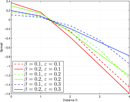
Figure 1 presents simulations for the options used in the counterexample above, i.e. µ1=2, µ2=3, and m=1, with different values of β and ε. In each of one million draws, the actual utilities u1, u2 are drawn from uniform distributions on {µi−1,µi,µi+1}. The ratings in Phases 1 and 3 and the choices in Phase 2 follow the model described above. Accordingly, in the simulations we obtain spreads for all possible values of D. Figure 1 shows that positive spread is observed for very small values of D, and negative spread is observed for larger values. Our previous counterexample corresponds to the values for D=2.
Figure 1: Simulation with two options, µ1=2, µ2=3, m=1, one million draws for each (β,ε) combination.
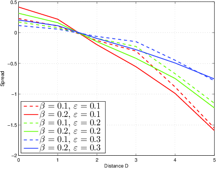
Figure 2 presents the results of simulations for a symmetric example where µ1=µ2=2 and m=1. These are the options used in the counterexample reported in Appendix A. Again, both positive and negative spread can be observed.
Finally, Figure 3 presents the average results of 60,000 simulated experiments with 80 possible options and 40 participants each. The preferences of the participants (i.e. the values uk) are generated randomly by first obtaining random values for µk according to a uniform distribution on the set {7,…,13}, then obtaining uk from a uniform distribution on {µk−5,…,µk+5}. Hence, realized utilities range from 2 to 18 and realized ratings in Phases 1 and 3 range from 1 to 19. In Phase 2, each participant is presented with 14 choices. A computer algorithm attempts to select two pairs each with distances D=0,1,… 6 according to the initial ratings (depending on the participant’s ratings, it might not always be possible to obtain 14 such pairs), in such a way that no option is used for two different choice pairs. The spread conditional on D is computed for each simulated experiment, and the figure presents average results over 10,000 experiments for each of six possible combinations of β and ε (the simulation took around 8 hours of computing time). As illustrated in the figure, the realized value of the spread Δ can be both positive (for small values of D) and negative (in this example, for D≥ 2). Note that the case D=0 replicates the results of Izuma and Murayama [2013] (who considered only D=0) for a different model.
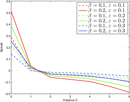
Figure 3: Average of 60,000 simulated experiments with 80 options, 40 participants, µk∈{7,…,13}, and m=5. 10,000 experiments for each (β,ε) combination.
It needs to be noted that FCP experiments inspired by cognitive dissonance theory typically rely on small values of D, since dissonance is generated by closeness to indifference (this would not necessarily be true if the motivation for an experiment arose from self-perception theory). In the simulations presented here, a value of D=0 always result in positive spreading. In any case, we remind the reader that whether a value of D indicates closeness to indifference or not depends on how fine the actual scale used in an experiment is. For a set of options as those in Figure 3, realized ratings vary from 1 to 19, and a distance of 2 (for which negative spreading is already observed) is rather “close”.
This section explains the mistake made in the proof in Chen and Risen [2010], which leads to the incorrect prediction of positive rating spread in the post-choice rating. Remember that one considers two fixed alternatives xi and xj such that ri1=rj1+D with D>0. The claim is that, using exclusively Assumptions 1, 2, and 3, it is possible to deduce that E[Δ|D]>0. In view of our counterexample and simulations above, this claim is incorrect.
The key mistake appears on p. 578 of Chen and Risen [2010], when the authors argue that because of (1), E[ri3−rj3|ri1−rj1=D]=D. In words, this says that, given the realized, possibly biased first rating difference, the expected second rating difference is equal to the first, biased one. This claim is incorrect in general.6
Consider the example detailed above, i.e., µ1=2, µ2=3, m=3, and
D=2, exactly as in our counterexample
in the previous section. We proceed to compute E[ri3−rj3|D=2].
E[r^3_i-r^3_j|D=2]=
Pr{r^1_j=0,r^1_i=2|D=2}E[r^3_i-r^3_j|r^1_j=0,r^1_i=2]
+Pr{r^1_j=1,r^1_i=3|D=2}E[r^3_i-r^3_j|r^1_j=1,r^1_i=3]
+Pr{r^1_j=2,r^1_i=4|D=2}E[r^3_i-r^3_j|r^1_j=2,r^1_i=4]
+Pr{r^1_j=3,r^1_i=5|D=2}E[r^3_i-r^3_j|r^1_j=3,r^1_i=5]
=β/2(1+β)(2-β/1-β-1)+1/2(1+β)(3-1/1-β)
+1/2(1+β)(4-5β/1-β-2)+β/2(1+β)(4-3-4β/1-β)
=2/1+β,
which is not equal to 2 for any 0<β<1/4, showing that the claim E[ri3−rj3|ri1−rj1=D]=D is incorrect.
To clarify matters further, consider an extreme case where µ1=2, µ2=3, and m=3 as above, but D=5. If the argument of Chen and Risen [2010] were to hold, we would have that E[ri3−rj3|ri1−rj1=5]=5. This is not true. Indeed, there is only one possibility for D=5 to be realized in our model, corresponding to ratings rj1=0 and ri1=5. This implies that uj=1 and ui=4 for sure. Hence,
E[ri3−rj3|D=5]=E[ri3−rjj|uj=1, ui=4] =E[ri3|ui=4]−E[rj3|uj=1]=4−1=3.Chen and Risen (2010, footnote 6) argue that it is equivalent to state Assumption 3 in terms of Pr{rkt>rℓt|uk>uℓ} or in terms of Pr{uk>uℓ|rkt>rℓt}. This is incorrect, but inconsequential for our analysis. Appendix B discusses this point and shows that our model also fulfills the additional assumption that 1/2 < Pr{uk>uℓ|rkt>rℓt}< 1.
The Appendix of Chen and Risen [2010] generalizes the approach considering a possible “regression to the mean” effect. In order to account for this possible effect, it is argued that instead of comparing the expected rating spread E[Δ|D] with 0, one should compare it with the quantity −R defined by −R=E[ri3−rj3|D]−D, which measures the expected increase of the rating difference in a hypothetical control group where participants rate twice without choice tasks in between. Chen and Risen [2010] claim that, with this adjustment, the FCP will exhibit rating spread strictly larger than the control group’s −R, even if the preferences are stable.
Of course, since this generalization includes the case R=0 as a particular case, it follows from our analysis above that the generalization is also incorrect. However, in this section we provide a more direct illustration.
Consider again our numerical example where u1 follows a uniform distribution on {1,2,3} and u2 follows a uniform distribution on {2,3,4} again. We compute the rating spread E[Δ|D] and compare it with E[ri3−rj3|D]−D for D=0.
Straightforward but cumbersome computations, analogous to the ones illustrated above, allow us to obtain the rating spread for D=0.
| E[Δ|D=0]= |
| (1−2ε). |
Similarly, we can compute E[r23−r13|D=0], which yields
| E[r23−r13|D=0]= |
| . |
According to Chen and Risen [2010], we should obtain that E[Δ|D=0]−E[r23−r13|D=0]>0. Straightforward computations show that
E[Δ|D=0]−E[r23−r13|D=0]=
| ⎡ ⎣ | (2−3β)(1−2ε)−(1−β) | ⎤ ⎦ |
which is smaller than zero for ε>1−2β/4−6β. Note that 1−2β/4−6β is smaller than 1/2 for any β<1/4. That is, when ε fulfills the condition above, the rating spread adjusted for the “regression to the mean” effect for D=0 in this numerical example is negative. Hence, the claim of Chen and Risen [2010] is still incorrect after adjusting for a “regression to the mean” effect.
Our simulations and those of Izuma and Murayama [2013] suggest that in the extreme case with D=0, positive spreading might occur in the absence of choice-induced preference change, i.e. the result stated by Chen and Risen [2010] might be correct in this particular case. This would be intuitive, because when D=0, if actual preferences are close to indifference, we would expect the rating difference in Phase 3 to be also close to zero, but if actual preferences are not close to indifference, the fact that an option is chosen is a signal on the actual preference and we would expect positive spreading. Intuitions, however, can be misleading, and hence we set out to provide a formal proof of this fact. Since the case D=0 is especially prominent in the literature, this proof is of independent interest.
The result we prove is not limited to our model. Rather, it applies generally to any model satisfying a few elementary assumptions. Those include Assumptions 1-2 from Chen and Risen [2010] (Assumption 3, interestingly, is not needed) and a new, minimal assumption dealing with knife-edge cases of exact indifference.
Formally, we consider any model where, given the true utilities, the random variables capturing ratings (in Phases 1 and 3) and choices are all independent. that is, although of course ratings and choices are derived from preferences, the corresponding error terms are independent. Further, Assumptions 1 and 2 are fulfilled, and the following assumption also holds.
Assumption 4: For each two alternatives xk, xℓ,
| Pr{uk=uℓ|rk1=rℓ1}<1. (-5) |
This assumption, which is fulfilled in our model, means that even if the observed ratings in the first phase are identical (D=0), it is not necessarily true that the options are actually indifferent. This does not follow from Assumptions 1-3, because those refer to strict preference only. It is, however, a natural consequence of the idea that ratings are noisy versions of preferences, and it is immediately fulfilled in our model.
Consider now the case D=0. That is, we consider only pairs such that ri1−rj1=0. We want to show that E[Δ|D=0]>0 using only Assumptions 1,2, and 4, rather than relying on a particular model.
To simplify the following equations, let pi=Pr{ui>uj|D=0}, pj=Pr{ui<uj|D=0}, and p0=Pr{ui=uj|D=0} denote the probabilities that xi is actually strictly preferred to xj, that xj is strictly preferred to xi, and that the two options are truly indifferent, respectively, all conditional on having observed equal ratings in Phase 1.
First we decompose E[Δ|D=0] with respect to the realizations of utilities as follows.
E[Δ|D=0] = p_i·E[Δ|D=0, u_i>u_j]
+ p_0·E[Δ|D=0, u_i=u_j]
+ p_j·E[Δ|D=0, u_j>u_i]
By Assumption 1, E[Δ|D=0, ui=uj]=0. That is, if the participant is truly indifferent, the expected difference in ratings is zero). Hence, the second term above is zero. Note that, if Assumption 4 did not hold, we would have p0=1 and hence E[Δ|D=0]=0. The remainder of the analysis hinges on Assumption 4, i.e. p0<1.
We now decompose the expression depending on the actual choices in Phase 2. Since D=0, we further simplify the spread by noting that Δ=ri3−rj3 if xi is chosen and Δ=rj3−ri3 if xj is chosen.
E[Δ|D=0]=
p_i(Pr{c(x_i,x_j)=x_i|D=0,u_i>u_j}·
E[r^3_i-r^3_j|D=0,u_i>u_j,c(x_i,x_j)=x_i]
+ Pr{c(x_i,x_j)=x_j|D=0,u_i>u_j}·
E[r^3_j-r^3_i|D=0,u_i>u_j,c(x_i,x_j)=x_j])
+ p_j(Pr{c(x_i,x_j)=x_i|D=0,u_i<u_j}·
E[r^3_i-r^3_j|D=0,u_i<u_j,c(x_i,x_j)=x_i]
+ Pr{c(x_i,x_j)=x_j|D=0,u_i<u_j}·
E[r^3_j-r^3_i|D=0,u_i<u_j,c(x_i,x_j)=x_j])
That is, the first of the two major terms (starting with pi) represents the case where xi is actually strictly preferred to xj, subdivided into the cases where xi is chosen and xj is chosen. Analogously, the second major term (starting with pj) corresponds to the case where xj is strictly preferred to xi, subdivided into the same cases.
Since, given the utilities, ratings are independent of the choices, we have that E[ri3−rj3|D=0,ui>uj,c(xi,xj)=xi]=E[ri3−rj3|D=0,ui>uj,c(xi,xj)=xj], because which option has been actually chosen in Phase 2 does not change the expectation of the ratings in Phase 3. Further, conditional on a given event, E[rj3−ri3]=−E[ri3−rj3]. Factoring out terms, we can simplify the expression as follows.
E[Δ|D=0]=
p_i·E[r^3_i-r^3_j|D=0,u_i>u_j] ·
(Pr{c(x_i,x_j)=x_i|D=0,u_i>u_j}
- Pr{c(x_i,x_j)=x_j|D=0,u_i>u_j})
+ p_j ·E[r^3_j-r^3_i|D=0,u_i<u_j] ·
(Pr{c(x_i,x_j)=x_j|D=0,u_i<u_j}
- Pr{c(x_i,x_j)=x_i|D=0,u_i<u_j})
Let us consider the terms in this expression separately. By Assumption 1, Ei=E[ri3−rj3|D=0,ui>uj]=ui−uj>0 and Ej=E[rj3−ri3|D=0,ui<uj]=uj−ui>0. By Assumption 2, Qi=Pr{c(xi,xj)=xi|D=0,ui>uj} − Pr{c(xi,xj)=xj|D=0,ui>uj}>0 (the probability of choosing an option is larger than the complementary if that option is actually the preferred one); analogously, Qj=Pr{c(xi,xj)=xj|D=0,ui<uj} − Pr{c(xi,xj)=xi|D=0,ui<uj}>0.
We have that
| E[Δ|D=0]=pi· Ei · Qi + pj · Ej · Qj |
Since by (-5) either pi or pj are strictly positive (and of course both are weakly positive) and we have just argued that Ei,Ej, Qi, and Qj are all strictly positive, it follows that E[Δ|D=0]>0. In conclusion, we have proven the following.
Theorem: For any model of random
utilities, ratings, and choices (where ratings in phases 1 and 3 and choices are independent given the utilities) fulfilling Assumptions 1, 2, and 4, the value of E[Δ|D=0] is strictly positive.
We conclude that positive spreading always obtains in the FCP for D=0, for a broad family of models. This result explains the simulation results of Izuma and Murayama [2013] and also our own simulations for the case D=0. Beyond that, it means that in any FCP study, if only pairs with D=0 are considered, one will obtain positive spreading even in the absence of preference change. However, as our previous counterexample shows, this result cannot be extended to the case D>0. If a model incorporates reasonable continuity assumptions, the result can obviously be extended to small values of D. However, whether a particular value of D>0 is small or large depends on the scale (recall, e.g., our simulation in Figure 3). Hence, the result above has limited bearing on studies with D>0 or on those using rankings (where exact indifference is excluded).
Analytical models and empirical/experimental studies are complementary. An analytical model of behavior should be based on a set of minimal, reasonable, uncontroversial assumptions. The formal implications of such a model should then be tested empirically. If experimental evidence systematically points towards an effect not predicted by the model, one has strong reason to believe that a feature of actual behavior has been uncovered.
We have presented a reasonable model built on very weak assumptions, which also fulfills the assumptions employed in Chen and Risen [2010]. We have shown that this model does not predict a systematically positive spreading in the free-choice paradigm (especially when D is larger than zero). This conclusion, of course, implies that the main claim of Chen and Risen [2010] is false, and we have pointed out one purely mathematical mistake in their proof. However, we have also shown that a small set of reasonable assumptions suffices to imply positive spreading (in the absence of preference change) for the particular case D=0.
What do we conclude from our analysis? Clearly, the free-choice paradigm is flawed, and Chen and Risen [2010] are to be credited with making this point explicit. The empirical observation of positive spreading using this paradigm in a specific study does not allow us to conclude that preference change has occurred. Our analysis, however, has further implications. We have shown that, although it is not true that the expected rating spread with immutable preferences is zero, it is not true either that it must be positive. Actually, even negative spreading might occur. As a consequence, failure to find positive spreading does not imply the absence of preference change. At a more abstract level, however, we observe that a reasonable model of behavior does not predict consistent positive spreading but positive spreading has been consistently observed for decades. We conclude that, taken in its entirety, experimental evidence from the free-choice paradigm (as long as data with D>0 was obtained) is indeed valuable and points towards an effect which still needs to be clarified, understood, and explained.
In other words, what our example shows is that not every reasonable model of immutable but noisy preferences will predict positive spreading. If previous studies just measured artificial spreading, originating on the biases in the FCP and not on actual attitude change, one would have expected frequent instances of negative spreading (unless, of course, all of them have been victims of publication bias). The most likely interpretation of the large body of evidence available at this point is that actual choice-induced attitude change exists, but has often been overestimated (and occasionally underestimated) due to the flaws in the FCP. Hence, in our opinion, empirically observed positive spreading remains informative, even if the basic effects in the literature need to be reestablished using improved paradigms.
We have kept our model, and especially our counterexample, as simple as possible. We see that the rating spread with immutable preferences hinges on the configuration of the behavioral model, for instance on the distributions of utilities and ratings, the description of the choice rule, and particularly, the predetermined rating difference D in Phase 1. Given specific assumptions on the choice heuristics, the distributions of utilities and ratings, and the scale of ratings, we see that when D is relatively large, the expected rating spread conditional on D is negative, and when D is relatively small, this spread is positive. A host of extensions and variants is of course possible. One could for example consider specific distributional assumptions on uk, or consider cases where the set of utility values is not restricted a priori, or the ratings are constrained to a strict subset of the actual utilities, or the ratings can differ from the utilities more than slightly. In view of our analysis, any such model will lead to positive spreading for D=0. Some particular models might lead to positive spreading for larger values of D. However, each of those alternatives and variants will contain specific additional assumptions which could and should be discussed on empirical and formal grounds. The point of a model developed around an experimental paradigm should be to help interpret and organize the data. There is an important difference between using a highly specified model to prove that a behavioral phenomenon is to be expected and using a particular case of a family of models as a counterexample to show that a claimed result is false in general.
We hope that this article has contributed to clarifying what we know and what we do not know on the biases built within the free-choice paradigm. In conclusion, the fact that expected spreading for specific rating distances and model specifications might be nonzero (positive or negative) makes improved experimental designs highly desirable. Examples include Chen and Risen [2010], Risen and Chen [2010], the blind-choice studies of Egan et al. [2010] and Sharot et al. [2010], and the implicit-choice paradigm of Alós-Ferrer et al. [2012]. This is the true value of the discussion started by Chen and Risen [2010]. However, the fact remains that experimental data point at positive spreading and models based on a minimal set of reasonable assumptions do not fully explain such spreading. Hence, taken as a whole, the trove of evidence delivered by dozens of previous experiments remains informative and should not be discarded lightly.
Of course, one counterexample suffices to establish the falsehood of a result. Here, however, we present a second counterexample within the framework of the general model in the main text in order to further clarify matters. Specifically, we strengthen the requirements on the counterexample by asking for a symmetric one where the involved alternatives are identically distributed, i.e., µk=µℓ=µ. That is, uk and uℓ follow the same (uniform) distribution with support V = {µ−m, …, µ, …, µ+m} (µ, m ∈ ℕ).
Specifically, let µ=2 and m=1; hence V={1,2,3}. Further, suppose that r21−r11≡ D=2. There are only three possibilities for r1 to yield D=2: r1=(0,2), (1,3), or (2,4). The choice probabilities are identical to the ones in the example in the main text.
Case 1: r1=(0,2). In this case,
Pr{u=(1,1)|r1=(0,2)}= Pr{u=(1,3)|r1=(0,2)}=β,
Pr{u=(1,2)|r1=(0,2)}=1−2β. Given the choice probabilities,
we have
Pr{c(x_1,x_2)=x_1|r^1=(0,2)}=
1/2 β+ε(1-β) ≡f(ε,β),
Pr{c(x_1,x_2)=x_2|r^1=(0,2)}=1-f(ε,β)
Using the terms above, we obtain
E[r^3_1-r^3_2|r^1=(0,2), c(x_1,x_2)=x_1]=
-ε/f(ε,β)
E[r^3_2-r^3_1|r^1=(0,2), c(x_1,x_2)=x_2]=
1-ε/1-f(ε,β)
Using these two results, we have
| E[Δ|r1=(0,2)]=−(1−2ε)(1−2β), |
which is smaller than 0 for any 0<ε<1/2 and 0<β<1/4.
Case 2: r1=(1,3). In this case,
Pr{u=(1,2)|r1=(1,3)}=Pr{u=(2,3)|r1=(1,3)}=
β(1−2β)/(1−β)2,
Pr{u=(1,3)|r1=(1,3)}=(1−2β)2/(1−β)2, and
Pr{u=(2,2)|r1=(1,3)}=β2/(1−β)2. Given the
choice probabilities, we can obtain
Pr{c(x_1,x_2)=x_1|r^1=(1,3)}=
1/(1-β)^2[1/2
β^2+ε(1-2β)] ≡g(ε,β)
Pr{c(x_1,x_2)=x_2|r^1=(1,3)}= 1-g(ε,β).
Using the terms above, we can derive
E[r^3_1-r^3_2|r^1=(1,3), c(x_1,x_2)=x_1]=
-2ε1/g(ε, β)1-2β/1-β,
E[r^3_1-r^3_2|r^1=(1,3), c(x_1,x_2)=x_2]=
2(1-ε) 1/1-g(ε, β)1-2β/1-β.
These imply
| E[Δ|r1=(1,3)]=− |
| β(1−2β)(1−2ε) |
which is smaller than 0 for any ε<1/2 and β<1/4.
Case 3: r1=(2,4). This case is symmetric to the
case r1=(0,2), and we find that
| E[Δ|r1=(2,4)]=E[Δ|r1=(0,2)]<0. |
Combining the three cases above, we have
| E[Δ|D=2]<0, |
which contradicts positive spreading.
The mathematical analysis in Chen and Risen [2010] contains an additional mistake. The authors argue that it is equivalent to state Assumption 3 in terms of Pr{rkt>rℓt|uk>uℓ} or in terms of Pr{uk>uℓ|rkt>rℓt} (see Chen & Risen, 2010, footnote 6). This claim is actually incorrect without additional assumptions. This is, in any case, inconsequential for our purposes, because, as observed in the main text, the main problem is an incorrect application of Assumption 1.
Even if one adopted this alternative version of Assumption 3, however, our counterexample would hold. This is because our model can also be shown to satisfy the additional assumption that 1/2 < Pr{uk>uℓ|rkt>rℓt}< 1. The argument that this conditional probability is smaller than 1 is identical to the one on Pr{rkt>rℓt|uk>uℓ} in the main text, because we argued on the joint probability. Showing that the probability is larger than 1/2 involves a more involved mathematical argument which we detail below. Essentially, it can be shown that this additional assumption is also fulfilled for arbitrary distributions of uk,uℓ if β is small enough. If specific distributions are assumed, sharper bounds on β can be obtained. Specifically, we show below that if every uk is uniformly distributed on Vk, then the assumption that Pr{uk>uℓ|rkt>rℓt}>1/2 is fulfilled for any β<0.21; alternatively, it is fulfilled for any β<1/4 under the slightly sharpened constraint that |µk−µℓ|<2m−1 for any two alternatives xk,xℓ.
First we establish that, for arbitrary utility distributions, the additional assumption Pr{uk>uℓ|rkt>rℓt}>1/2 will be fulfilled for β small enough. Since β is a noise parameter thought to be small, this is actually enough to establish the argument. However, we will also show below that specific bounds can be found for specific distributions.
Since ratings are generated as perturbations of the realized
utilities, in our model it is easy to compute
Pr{u_k>u_ℓ, r^t_k>r^t_ℓ}=
Pr{u_k=u_ℓ+1}((1-β)^2+2β^2)+
Pr{u_k = u_ℓ+2}(1-β^2)+ Pr{u_k≥u_ℓ+3}
and
Pr{u_k≤u_ℓ, r^t_k>r^t_ℓ}=
Pr{u_k=u_ℓ}(2β-3β^2)+Pr{u_k=u_ℓ-1} β^2.
Note than the latter probability converges to zero as β→ 0
while the former converges to Pr{uk≥ uℓ+1}, which is
not zero because |µk−µℓ|≤ 2m−1. Consequently, by
choosing the noise parameter β small enough, we obtain that
Pr{u_k>u_ℓ, r^t_k>r^t_ℓ}>Pr{u_k≤u_ℓ,
r^t_k>r^t_ℓ},
which in turn implies Pr{uk>uℓ|rkt>rℓt}>1/2.
Suppose now that uk,uℓ follow uniform distributions on Vk,Vℓ. We aim to establish when equation (8) above holds, using expressions (8) and (8). Regrettably, the argument is mathematically cumbersome.
We distinguish three cases, µk = µℓ, µk > µℓ, and µk < µℓ. If µk = µℓ, the assumption of uniform distributions yields
|
and substituting in (8) we obtain that the assumption holds if and only if
| P1(β)=(8m+4)β2−(8m+2)β+2m2+m>0. |
This polynomial reaches its minimum at β=(4m+1)/4(2m+1)>(1/4), hence it is strictly decreasing for 0≤ β≤ 1/4. It follows that (8) holds for all 0 < β < 1/4 if and only if P1(1/4)≥ 0. A computation shows that P1(1/4)= 2m2−1/2 m−1/4, which is strictly positive for all m≥ 1. The conclusion follows.
Consider now the case µk > µℓ; let µk=µℓ+n
with n ∈ {1,2,..., 2m−1}. Slightly more involved computations
show that, for uniform distributions,
Pr{u_k=u_ℓ+1}= 2m+2-n/(2m+1)^2
Pr{u_k=u_ℓ}= 2m+1-n/(2m+1)^2
Pr{u_k=u_ℓ-1}= 2m-n/(2m+1)^2
Pr{u_k=u_ℓ+2}= 2m+1-|n-2|/(2m+1)^2
Pr{u_k ≥u_ℓ+3}= 1/(2m+1)^2( (n-1)(2m+1)
-(2m+1-|n-2|)
+1/2(2m-1+n)(2m+2-n))
and substituting in (8) we obtain that, for n=1, the
assumption holds if and only if
| (8m+4)β2−(8m+2)β+(m+1)(2m+1)>0. |
This polynomial has a minimum at β= 4m+1/8m+4>(1/4) and, by the same argument as in the previous case, the conclusion will follow if and only if P2(1/4)≥ 0. A computation shows that P2(1/4)=2m2+3/2 m+3/4, which is larger than zero for any m ≥ 1. Similarly, for n ≥ 2, the assumption holds if and only if
P3(β)=(8m+6−4n)β2−(8m+6−4n)β+
| (2m+2−n)(2m−1+n)+(n−1)(2m+1)>0. |
Again this polynomial has a minimum at β=1/2>1/4 and, by the same argument as in the previous case, the conclusion will follow if and only if P3(1/4)>0. A computation shows that P3(1/4)=−1/2 n2+(9/4+2m)n+(2m2−1/2 m−9/8) and this expression is larger than zero provided 9/4+2m−Q/2<n<9/4+2m+Q/2 with Q=√32m(m+1)+45/4; this condition is fulfilled because 1≤ n ≤ 2m−1, and the conclusion follows.
Last, consider the case µk < µℓ; let µk=µℓ−n
with n ∈ {1,2,..., 2m−1}. For uniform distributions,
Pr{u_k=u_ℓ+1}= 2m-n/(2m+1)^2
Pr{u_k=u_ℓ}= 2m+1-n/(2m+1)^2
Pr{u_k=u_ℓ-1}= 2m+2-n/(2m+1)^2
Pr{u_k=u_ℓ+2}= 2m-1-n/(2m+1)^2
Pr{u_k ≥u_ℓ+3}= (2m-1-n)(2m-2-n)/2(2m+1)^2
and substituting in (8) we obtain that the assumption
holds if and only if
P_4(β) = 2(4m-2n+1)β^2-2(4m-2n+1)β+
1/2 (2m-n)(2m+1-n)>0,
where 4m−2n+1>0 and (2m−n)(2m+1−n)>0. Again this polynomial has
a minimum at β= 1/2>1/4 and, by the same argument as in the
previous cases, the conclusion will follow if and only if
P4(1/4)≥ 0. A computation shows that P4(1/4)=1/2
n2−(2m−1/4)n+2m2−1/2 m−3/8. This expression is
strictly larger than zero if n<2m−1+√13/4 or
n>2m+√13−1/4. The former holds whenever n≤
2m−2, and hence we conclude that the assumption holds for any
0<β<1/4 under the sharpened condition that
|µk−µℓ|<2m−1 for any two alternatives xk,xℓ. If
this is not assumed, we need to determine when the condition holds
for the extreme case n=2m−1. In this case, the condition
P4(1/4)≥ 0 reduces to 6β2−6β+1≥ 0, which holds
if β≤ 1/2−(1/6)√3∼ 0.211. Hence, the assumption
always holds (without sharpening the original condition
|µk−µℓ|≤ 2m−1) for β ≤ 0.21.
Copyright: © 2014. The authors license this article under the terms of the Creative Commons Attribution 3.0 License.
This document was translated from LATEX by HEVEA.