Why are gainers more risk seeking

The phenomenon that prior gains may increase people’s willingness to accept risky gambles is named as the house money effect (Thaler and Johnson, 1990). Many studies have shown that the “house money effect” is a robust phenomenon but few scholars explain the mechanism of it well. We suppose the reason for the house money effect is that the ante (starting amount) is from the prior gambling profits, and its potential loss has relatively low psychological value. To test this hypothesis, we designed a series of studies using two-stage gambles. A total of 915 university students participated. In Study 1, in addition to a standard condition (which replicated the basic effect), we test how people respond to “prospect theory, with memory” frame, a “concreteness” frame and “quasi-hedonic” editing. None of these types of frames result in a significant house money effect. In Study 2, we certify the reference point shift to 100 Yuan in the second-stage gamble, thus the house money effect can be regarded as the absence of loss aversion; Study 3, consisting of 3 sub-experiments, indicated that gambling profits and normal income will open different mental accounts which are spent quite differently. The pain of losing 100 Yuan allowance is more serious than that of losing 100 Yuan gambling wins. People will typically reject the gamble of 50/50 chance to gain or lose 100 Yuan if the ante is from the “normal income account”, but accept if the ante is from the “windfall account”. The results of the series of experiments prove the accuracy of our hypothesis mostly.

Keywords: The house money effect, Two-stage gambles, mental accounting, windfall.

1 Introduction

Loss aversion is one of the basic characteristics of decision making behavior. Kahneman and Tversky (1979) suggested people would typically reject gambles which offer a 50/50 chance of gaining or losing the same amounts of money because losses might generate bigger psychological utility than equivalent gains (Kahneman & Tversky, 1984; Kahneman, Knetsch, & Thaler, 1991; Ariely, Huber, & Wertenbroch, 2005). Previous studies documented that loss aversion was a widespread and robust phenomenon, and not only for money, but also for chocolates, lottery tickets, buildings and other items (Carmon & Ariely, 2000; Knetsch, 1989; Sasaki et al., 2008). However, the principle of loss aversion cannot explain some phenomena. For example, you probably may reject a gamble game showing a 50/50 chance of gaining or losing $100 because of loss aversion, but, if you are told that you have played once and won $100, do you want to bet now? Previous studies reported that under some circumstance a prior gain could increase people’s willingness to accept risky gambles. Some scholars named this phenomenon as the sunk gains or the house money effect (Laughhunn & Payne, 1984; Thaler & Johnson, 1990; Ackert, Charupat, Church, & Deaves, 2006; Harrison, 2007).

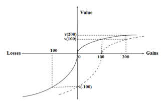
What is the underlying mechanism of the house money effect and how do prior gains result in risk seeking? Thaler and Johnson (1990) made an analysis based on the Prospect Theory (Kahneman & Tversky, 1979). According to the model, the prospects of options can be defined as V=Σπ(p)v(x). Kahneman and Tversky (1979) believed people would typically choose options that had brighter or better prospects. π(p) in the model represents the subjective assessment of probabilities of outcomes. Small probabilities are often overweighted (π(p)>p), while medium or high ones are often underestimated (π(p)<p); v(x) denotes the psychological utility. People’s cognition of gains or losses is relative to the reference point, rather than from the absolute level of wealth. Gains and losses are evaluated differently because of the shape of value function, which is concave in the gain area and convex in the loss area, reflecting the principle of diminishing sensitivity, so that |v(2x)| is smaller than twice of |v(x)|, in either direction. The loss function is steeper than the gain function, implying that decision makers are more sensitive to losses than gains (| v(x)|<| v(−x)|), see Figure 1. For the current gamble “if you have played once and won $100, do you want to continue or not?” If participants edit the second-stage gamble as depending on the prior gains, which Thaler and Johnson (1990) labeled as “Prospect theory, with memory” editing, the game may be rewritten as “option A, you quit and you get $100 for sure; option B, you have a 50% chance to get $200 and a 50% chance to get nothing”. Since π(1/2)<1/2, π(1)=1, and 2v(100)>v(200), V(A)=π(1)v(100)>V(B)=π(1/2)v(200). Therefore people should typically choose option A—rejecting the option to play again. If the second-stage gamble is seen as independent, which was named as “concreteness” editing (Thaler & Johnson, 1990), this gamble may be described as “option A, you quit and you will win or lose nothing; option B, you have a 50% chance to get $100 and a 50% chance to lose $100”. Because | v(−100)|>v(100), V(B)=π(1/2)[v(100)−| v(−100)|]<0=V(A). Participants should also typically reject this game. Thaler and Johnson’s (1990) explanation of the house money effect was that people complied with quasi-hedonic editing rules and tended to segregate gains and integrate later losses with the prior gains (if later losses were no bigger than prior gains). So this game may be framed as “option A, you quit and you will get $100 for sure; option B, you will have a 50% chance of getting $100, and later on you will get another $100 and there is also another 50% chance you will get or loss nothing”.

Although quasi-hedonic editing could in principle lead to less loss aversion (since 2v(100)>v(200)), some important issues remain to be resolved. Firstly, Thaler and Johnson summarized the quasi-hedonic editing rule based “S” shaped value function curve and experimentally demonstrated that quasi-hedonic editing leads to a larger psychological value. For example, Mr. A, who won $50 in one lottery and $25 in the other, might feel happier than Mr. B, who won $75 in just one lottery. However, Thaler and Johnson failed to directly test whether people really framed successive results of decision making in that way. Secondly, Thaler and Johnson claimed that quasi-hedonic editing resulted in the house money effect, but they did not test how people responded to this frame. Thirdly, how people frame the second-stage gamble actually reflects a different set of reference points. In the current example, in the case of concreteness editing, the current state of owning $100 is regarded as the reference point (the dotted curve in Figure 1), whereas, in the case of “Prospect theory, with memory” editing, $0 is regarded as the reference point (the solid curve in Figure 1). In the case of quasi-hedonic editing the reference point is regarded as being dynamic, which in the second-stage gamble might be zero for a loss, or $100 for a win. However, Thaler and Johnson did not ascertain how the reference point shifted in subsequent decision-making. In addition, based on the quasi-hedonic editing, there is no perceived “loss” in the second-stage gamble (if subsubsequent losses are no bigger than prior gains) since the “loss” are just coded as “a reduction of gains”. This should result only in the decrease of positive consequence like positive emotion, but not the appearance of negative consequence as negative emotion, since the state is always above the reference point. For the current case, if the second-stage gamble is a loss, the result is coded as “the gains decrease from $100 to zero” so one should feel “placid” for the result. In another example, “you have gained $800 and then lose $100”, the result of loss is coded as “the gains decrease to $700” and you should feel “happy” for the “loss”, an unlikely outcome.

Arkes, Hirshleifer, Jiang and Lim (2008) explored how the reference point shifted following gains or losses. In their studies, they asked participants to state today’s stock price that would generate the same utility as a previous change (gain or loss) in the stock price. From participants’ responses, they calculated that people found it easier to adapt to gains than to equal-sized losses. Arkes, et al., provided a replication of the asymmetric adaptation of gains and losses and suggested that the reference point adaptation was larger for Asians than for Americans (Arkes, Hirshleifer, Jiang & Lim, 2010). Based on the Study of Arkes, et al (2008), we believe that, in the second-stage gamble, the reference point does shift to $100. So, if it is a win, the result can be edited as “get another $100”; if a loss, the result can be edited as “lose the prior gained $100”. The key point to explain the house money effect is how people feel about “the loss of prior gained $100”. The house money effect essentially reflects the reduced loss aversion.

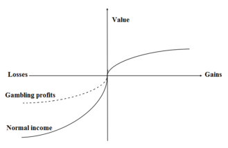
The ratio between gain and loss that can make gain and loss equivalent in psychological utility is called the index of lose aversion. Previous studies reported the index was usually between 2 to 2.5 (Kahnema, Knetsc & Thale, 1991; Tversky & Kahneman, 1992; Abdellaoui M, Bleichrodt H & Paraschiv C, 2007). Some scholars considered that emotional attachment generated loss aversion (Carmon et al., 2003; Kermer et al., 2006; Liu, Liang & Li, 2009). Kahneman & Tversky (1979) showed that loss aversion phenomenon was more serious when the ante (starting amount) was higher. Strahilevitz & Loewenstein (1998) also documented greater loss aversion for commodities with more extension of ownership and more emotional attachment: the loss of belongings with higher psychological value generates more intense negative emotions, thus leading to the loss curve getting steeper. We suggest a hypothesis that the slope of loss curve is flexible; it may get both larger and smaller. In the case of winning, people tend to regard gambling yield as unexpected fortune with relatively low psychological value. The loss of such windfall gains will induce less negative emotion, in other words, the loss curve of gambling profits is less steep than that of normal incomes, so the index of loss aversion is also smaller, as shown in Figure 2. Loss aversion will disappear if the index is smaller than or equal to 1.

Thus, we hypothesize that normal incomes and gambling profits essentially reflect different mental accounts. The theory of mental accounting (Thaler, 1980, 1985; Kahneman & Tversky, 1979) holds that people have an implicit system of accounting, which leads them to violate expected-utility theory as applied to overall wealth (Thaler, 1985). People appear to maintain mental accounts for different sources, uses and ways of storage, and treat each account differently (Thaler, 1985). Mental accounts are settled depending on the sources of wealth, like normal incomes, windfall, etc. (Kivetz, 1999). Money won in a lottery is likely to be spent very differently from money obtained from regular income, even if the amount and the timing of receipt from these two sources were identical (Rajagopal & Rha, 2009). Arkes, et al. (1994) suggested windfall gains are spent more readily than other types of assets, since windfall gains have less psychological value. Mental accounting mainly works through the non-fungibility effect: individuals will distribute money into different mental accounts, which have different functions and uses and cannot be replaced by each other (Thaler, 1985).

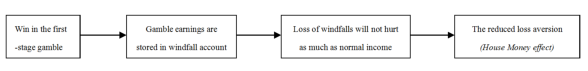
To summarize, we hypothesize that the process leading to the house money effect, as shown in Figure 3, is that (1) people set special mental account for gambling earnings as windfall gains and (2) people are more willing to accept risky gambles in windfall gains accounts than normal income accounts, because the loss of windfall gains will not hurt that much.

2 Study 1

Study 1 was designed to test how people would respond to the “prospect theory, with memory” frame, quasi-hedonic editing frame and concreteness frame, in addition to replicating the house money effect with the standard frame for a 2-stage gamble.

2.1 Participants and procedure

The participants were 380 male undergraduates from a military medical university of China, with a mean age of 20.23 years (SD =1.54), who agreed to take part in the study for extra course credit. There were several advantages for recruiting these special participants. Firstly, their professions have nothing to do with economics. Secondly, their tuition and living expenses are provided by the government and their parents generally don’t give them extra money. So their incomes are relatively equivalent. Thirdly, previous studies documented substantial gender difference in financial decisions involving risk (Barber & Odean, 2001; Eriksson & Simpson, 2010), so we recruited just male participants.

Here we using a between-participants design, 380 male undergraduates were randomly assigned to 4 groups labeled as a₁₋₄. Each participant completed only one question. Participants were told there was no right or wrong answer, and that the study was anonymous and without a time limit.

2.2 Results

Table 1 presents the response of participants to four different frames. Most participants of a₂, a₃ and a₄ choose the conservative option (χ²a₂(1, 95)=20.167, p<0.001; χ²a₃(1, 96)=10.116, p=0.001; χ²a₄(1, 94)=12.298, p<0.001). But there is no such a significant difference in the number of people choosing conservative or risky option in group a₁ (χ²(1, 95)=0.095, p=0.785). In other words, risk aversion is seen under the quasi-hedonic frame, the “prospect theory, with memory” frame and concreteness frame, but not under the standard frame of the house money effect. There is a significant between-groups difference in willingness to take risks, with higher gamble frequency among participants from group a1 (χ²(3, 380)=14.213, p<0.01). The comparison of conditions a₁ and a₃ replicates the basic house money effect (chi²(1)=5.51, p<.02).

2.3 Discussion

Participants of group a₁₋₄ essentially face the same choice: “Risky option—you will have 50% chance getting ¥200, and 50% chance getting nothing; conservative option—you will get ¥100 for sure”. Situations a₂₋₄ respectively framed the second-stage gamble as a dependent or independent event with the previous gains, or according to the quasi-hedonic editing rules that people tend to segregate gains and integrate later losses with the prior gains. But risk aversion is significant in all groups of a₂₋₄. “Prospect theory, with memory” editing and concreteness editing should lead to risk aversion in theory as analyzed in the introduction. Quasi-hedonic editing could in principle lead to less risk aversion; however the results of Study 1 suggested that quasi-hedonic editing does not generate the house money effect. So another explanation is needed.

Based on the theory of reference point adaptation (Arkes, et al, 2008), people easily adjust to prior gains. If that is the case, then a subsequent potential loss will be regarded as a “loss” but not as a “reduction of gain”. Since gambling earning comes easily, people may regard such money as windfalls. Arkes, et al (1994) documented that windfall gains were spent more readily and (hence) with less psychological value. We thus suggest that the house money effect may be explained in this way: In the case of winning, people tend to set a special account as windfall for the earnings. In the second-stage gamble, the ante is taken from the special account, and it is easier for people to accept the potential loss of windfall, thus participants become more risk seeking. For proving the hypothesis we have to verify the following two key points: (1) the reference point does shift to ¥100 in the second-stage gamble—this is the primary goal of Study 2—and (2) people open a special account for gambling winnings as windfall gains—the primary goal of Study 3.

3 Study 2

3.1 Participants and procedure

The participants were 80 male postgraduates (24.36±1.06 years old) majoring in clinical medicine who agreed to take part in the study for a notebook as a gift.

Participants were randomly assigned to 2 groups labeled as b₁₋₂. Questionnaires of b₁ and b₂ each consisted of three questions and were designed to test whether the reference point shifts. Question 1 asked participants to judge their emotional responses to the result of the second-stage gamble; Question 2–3 inquired about participants’ comprehensions to the result of second-stage gamble and the final result of the two-stage gamble. We gave two possible comprehensions for each question based on the hypotheses that the reference point was at ¥100 or at ¥0, which were labeled as comprehension A and comprehension B (Table 2 and Table 3). The responses were made on a 6-point Likert scale ranging from 1 (strongly tend to comprehension A) to 6 (strongly tend to comprehension B). Similar to a simple dichotomous scale where a participant would choose one of the two treatments, participants using a 6 point-scale must also favor one procedure over the other, since there is no mid-point. (Choices 1–3 imply a preference for prefer comprehension A; 4–6, a preference for B.) In addition, the 6-point scale allowed us to determine the strength of the choice preference (Bruine de Bruin, Parker, & Fischhoff, 2007). To balance the effects of question order, we created two versions: in version A, participants answer their comprehensions to the result of second-stage gamble first, then their comprehensions to the final result of two-stage gamble; in version B, the reverse.

3.2 Results

We hypothesize that the reference point shifts to ¥100. Thus people’s cognition about the results of the second-stage gamble should be relevant to ¥100 but not any others. As illustrated in Table 2, 97.5% of the participants answered that they would be happy if if they win in the second stage gamble. Significant more people tend to edit “the result of win in the second stage gamble” as “win anther ¥100” than as “the gains increase from 100 to 200” (χ²(1, 40)=6.40, p=0.011). The mean response is almost significantly less than 3.5, which is the theoretical mid-point of the 6 point-scale (t₃₉ = −1.99, p=.054), indicating that people prefer comprehensions A than B. As for the understanding of the final result of the two-stage game, there is no significant difference in the number of people choosing comprehensions A or B (χ²(1, 40)=2.46, p=0.12). There is also no significant difference between the mean response and the theoretical mid-point (t39=−.47, p=.64). The difference between the mean responses of Question 2 and Question 3 is not significant (t39=−1.08, p=.28).

As illustrated in Table 3, 87.5% of the participants answered that they will be unhappy if they lose in the second-stage gamble. Significantly more people tend to edit “the result of loss in the second stage gamble” as “loss the prior gained ¥100” but not “the gained money decreased to zero” as suggested by Thaler & Johnson (1990) (χ²(1, 40)=14.40, p<0.001). The mean response is significantly less than 3.5 (t₃₉=−4.79, p<.001). Significantly more people tend to integrate losses with prior gains when considering the final result of the two-stage gamble (χ²(1, 40) =15.24, p<0.001). The mean response is also significant larger than 3.5 (t₃₉=5.05, p<.001), suggesting that people prefer comprehensions B to A. The difference between the mean responses of Question 2 and Question 3 is significant (t₃₉=−8.34, p<.001).

3.3 Discussion

The results of Study 2 demonstrate the reference point shift to ¥100 when considering the result of the second-stage gamble. People tend to regard the result of a win as “another gain of ¥100” and the result of a loss as “the loss of prior gains”. So the house money effect can be regarded as the reduced loss aversion. However, it seems that there is a tendency for the reference point to shift back to zero for participants when evaluating the final results of the two-stage gamble, especially for those who lose in the second-stage gamble. The result of Question 3 to some extent supported the quasi-hedonic editing rule: The integration with prior gain of subsequent loss is greater than subsequent gain, when considering the final result of multi-stage decision making.

4 Study 3

The goal of Study 3 was to ask whether people set different mental accounts for normal income and gambling profits, and if they regard gambling profits as windfall gains. Three related hypotheses are relevant: (1) according to Arkes, et al. (1994), windfall gains have lower subjective value than other gains, thus the loss of such money will led to less negative consequences like negative emotion; (2) gambling earnings should be spent very differently than money obtained from regular income, since they are stored in different mental accounts, which may have different uses; (3) if there are different accounts for gambling earnings and normal income, then these two accounts should be non-fungible.

4.1 Participants and procedure

80 postgraduates (24.34±1.26 years old) were randomly assigned to two groups labeled as c₁₋₂ and 382 male undergraduates (20.43±1.54 years old) were randomly assigned to four groups labeled as D₁₋₂ and E₁₋₂. Participants received course credit or notebooks for their participation.

Questionnaires c₁₋₂ were adopted from previous studies (Eriksson & Simpson, 2010; McGraw, Larsen, Kahneman & Schkade, 2010), which found more apparent loss aversion with a unipolar scale than a bipolar scale. In group c₁₋₂, participants were asked to evaluate their emotional response strength of accidentally losing ¥100 gambling earning or ¥100 normal income. Responses were made on a 5-point Likert scale, from “1” expressing “placid” to “5” representing “extremely unhappy”; d₁₋₂ aimed to test the different willingness to spend money on a luxury tie; E₁₋₂ were designed to study the different willingness to accept the second-stage gamble in different mental accounts.

4.2 Results

The results show that losing ¥100 gambling profits will induce 2.33 units of negative emotion which is significantly smaller than the 3.25 units of negative emotion brought by the loss of ¥100 allowance (t₇₈=−3.58, p=.001).

Table 5 shows that, although most participants don’t want spend ¥800 (almost the total monthly income of cadets in China) on a tie, there is still a significant difference of proportions between d₁ and d₂ (χ²(1, 192)=20.281, p<0.001). There are significantly more participants who are willing to purchase luxury goods with gambling profits than normal income.

Table 6 shows the reversal of willingness to participate gambles with the change of mental accounts as a function of the ante. When participants are asked whether to bet with the previous gained ¥100 from the gamble, nearly half (46.3%) of them answer “yes”; but when the ante are changed to ¥100 allowance, only 31.6% of the participants want to continue, significantly less than 50% (χ²e₂=12.895, p<0.001). A chi-square test confirms that the difference between group d1 and d2 is significant (χ² (1, 192) =4.338, p<0.05).

4.3 Discussion

In Study 3, we firstly show that people will experience stronger negative emotion from losing a ¥100 allowance than from gambling gains. We also show that people are more willing to spend gambling earnings than normal incomes on an unattractive consumer item such as a luxury tie. Money earned from a gamble is spent quite differently from normal income since it is stored in a different mental account, with different purposes. Finally we test the non-fungibility effect between normal income and gambling earning. Participants of groups e₁ and e₂ actually face the same problem: after winning in the first-stage gamble, participants have ¥200 going into the second-stage. ¥100 must be taken out for a birthday present for Mother, and participants are asked whether they want continue to bet with the remaining ¥100. The response of groups e₁₋₂ are quite different. In group e₁, the taken out ¥100 is labeled as “allowance” and the remaining ¥100 is labeled as “gambling earnings”, and we don’t find significant risk aversionl. In group e₂ the taken out ¥100 is labeled as “gambling earnings” and the remaining ¥100 is labeled as “allowance”, and then participants were risk averse and most of them did not want to bet again. The results not only show that gambling earnings and normal incomes are stored in two different mental accounts, which are non-fungible with each other, but also that the house money effect appears only if the ante is from prior gains, which is the real cause for this phenomena.

5 General discussions

The current study replicates and extends previous work by Thaler and Johnson (1990) to address the mechanisms underlying the finding that prior gains increase willingness to accept risky gambles. We did 3 related studies consisting of 5 sub-experiments to test our hypothesis: The reason for people becoming risky in gambles after winning is that the ante is from the gambling earnings, which are regard as windfall gains and have relatively low psychological value, so that the loss of such money doesn’t hurt much. The findings strongly support the hypothesis.

5.1 The editing rules and reference point shift

Thaler and Johnson (1990) explained the house money effect based on the quasi-hedonic editing rules: people tended to segregate gains and integrate subsubsequent losses with prior gains (the integration can be achieved only if the original gains are no less than subsubsequent losses). However, according to this theory, subsubsequent losses should be regarded as the “decrease of gains”. Psychological feeling of loss does not exist, because the state will be always above the reference point. Thus the result of loss in the following gambles cannot cause any negative consequences, such as negative emotions. However, this idea is inconsistent with our regular experience and the conclusions of Study 2. For the case of “gain ¥100 in the first-stage gamble and then loss ¥100 in the second stage”, people tend to comprehend the result of the second-stage gamble as “loss the prior gained ¥100” but not “the gains decrees from ¥100 to zero”. It is a negative event, which can induce negative emotion; Our results also indicate that people perceive winning in the second-stage gamble as “win another ¥100” but not “the gained money increases from ¥100 to ¥200”. The current result is consisting with Arkes, et al.’s (2008) reference point adoption theory: It is easy and quick for people to adopt a gain as the references. So whether to bet in the second-stage gamble is decided by the competition between the eager to “win another ¥100” and the fear of “losing the prior gained ¥100”. We conclude that the house money effect essentially reflects a reduction or elimination of loss aversion.

The discussion of the reference point shift is not the main purpose of the current paper. At the same time, we also do not aim to deny the existence of quasi-hedonic editing. On the contrary, to a certain extent, our results support the existence of quasi-hedonic editing. We find that the editing rule of integrating subsequent loss with prior gains does exist when people consider the final result after two stages gamble. We feel that this editing rule works as a self-protection mechanism. For example, when loss in the second-stage gamble, people may comfort themselves: “Overall I don’t have any loss”. In other words, the reference point is at ¥100 when making decision, then comes back to zero if there is a loss, to reduce the hurt caused by loss. The other editing rule of segregating gains works when people consider the result of the second-stage gamble but not the final result. We suppose segregating gains can maximize positive psychological utility, and integrating gains may increase the sense of accomplishment and help decision makers determine whether expectations has been achieved, working together to influence people’s cognition about the final result of winning twice. However, all hypotheses remain speculative and how reference points shift in subsequent decision making is an interesting question for more future researches.

5.2 The metal account of windfalls

We believe gambling profits and normal income will open different mental accounts, and test the hypotheses in three respects. Firstly we show that people experience stronger negative emotion to losing a ¥100 allowance than a ¥100 gambling gain. This is consist with Arkes, et al. (1994), who argued that windfall gains had lower subjective value than equivalent non-windfalls so people would feel less painful from losing ¥100 in gambling earnings as from losing a ¥100 allowance. Soman & Cheema (2001) also found a similar phenomenon in their study on the sunk cost effect: when people spend the money from a windfall, it seemed easy for them to ignore the past inputs, so the sunk cost effect would be reduced or even disappear; but, when people spend the money from normal incomes, they will feel painful for the abandonment of the existing investment, and thus the sunk cost effect will be more serious.

According to our analysis, gambling profits and normal income will open different mental accounts, which must have different uses. The results of the luxury-tie purchase experiment of Study 3 supported our hypothesis: despite the unwillingness of most subjects, there are still more subjects who wish to purchase luxury ties with gambling earnings than normal incomes. Kivetz (1999) divided mental accounts into normal earning and windfall by the different sources of funds. Normal earning is generally used for saving or commodity expense; but windfalls tend to be used for luxury consumption or enjoyment (Henderson & Peterson, 1992; Thaler & Johnson, 1990). Li, Ling, Fang & Xiao (2007) concluded that, for Chinese people, the primary categories for the use of normal incomes were, in order, saving, relationship expenses, and expense for self development, while the corresponding categories for windfall gains were relationship expenses, saving and enjoyment. Allowance is stored in the mental account of normal incomes and gambling profit is stored in the windfall account, so their expense intention is quite different. Finally we showed that loss aversion disappears only if the antes were from the gambling incomes, through the manipulation of mental accounts. This experiment also found that normal incomes and windfalls will open different mental accounts that are non-fungibile.

Our study extends the work of Arkes, et al. (1994) and associates it with the theory of reference point adoption (Arkes, et al., 2008), which can help to explain the mechanism underling the house money effect: When winning, people are easily adapted to the gains such that their subsequent decisions are based on the current, but not the original, state. Usually, gambling games of zero-expectation are unattractive, since the pain of loss is greater than the bliss of an equivalent gain (| v(−x)|>v(x), x>0). However, gamble earnings come easily, thus the loss of such windfalls will not hurt as much (Arkes, et al., 1994), in other words, | v(−x)| > | v^′(−x)| (where v^′(−x) means the subjective value of losing x windfalls). With the decreases of the hurt caused by losses, the eagerness for participants to engage in the once unattractive zero-expectation games increases. We believe this is the psychological process that results in the house money effect.

5.3 Limitations and advice for future study

Besides the editing rules by Thaler and Johnson (1990) and our suggested interpretation of mental accounting of windfall gains, there are other potential explanations for the house money effect. For example, prior gains can create positive emotional reactions. Johnson and Tversky (1983), in their emotional generalization hypothesis, proposed that people are more likely to forecast higher potential risks when they are in a negative mood, whereas when they are in a positive mood, they are more likely to forecast lower potential risk events, which could explain risk-seeking behavior after making a profit. Moreover, prior gains may cause the “hot hand effect” (Gilovich, Valone, & Tversky, 1985), participants might feel that they were very lucky on a particular day and that their chances of winning are higher than the stated 50%. Both these explanations make some sense, but neither can explain our result of the non-fungibility test in Study 3. Participants of e₁₋₂ were both asked to image they had won in the first round. These hypotheses imply that their estimate of winning chances in the next round, as well as positive emotions, should be the same. But there is still a significant difference between the willingness to bet. But our result cannot exclude the potential influence of emotion or “hot hand effect” caused by prior gains; perhaps they are also some of the many reasons leading to the house money effect.

The present studies support two conclusions: (1) people still regard the loss of prior gains as an actual loss and not a reduction of profits, so it can cause negative results, such as negative emotions; (2) people would not feel too much hurt when they lose the gains of gambling, because such gains are considered as unexpected earnings. This, we think, is the true cause of the house money effect. However, in spite of this study’s contributions, there are still some limitations. The most import issue is that the gamble of 50:50 chance of winning or losing ¥100 is unattractive, but we ask participants to imagine that they have played once and won ¥100, and then inquire whether they want to continue.

Perhaps the second-stage question seemed odd to participants whose preferences would have led them to reject the symmetric gamble in the first stage, and who would therefore never have arrived at the second stage. It is possible that such participants would have responded to the second-stage gamble not with their own preferences, but rather with the imagined preferences of someone who would have accepted the first-stage gamble (and who would therefore be more likely to accept an identical gamble in the second stage). If so, such reasoning could lead to the appearance of a house money effect for reasons unrelated to participants’ actual preferences. However, this argument seems to assume that participants are processing the questions rather deeply, which may be usually not the case (e.g., some of the Thaler and Johnson (1990)’s results indicate that participants are not very active in their editing of prospects).

Moreover, when inquired about the will to bet after participating once, participants may keep the implicit commitment to participate, in other words, we would fail to differentiate the effect of prior participation and prior gains on people’s willingness to accept risky gambles. To clarify this issue, we conducted a small experiment in which 90 postgraduate students were recruited as participants and randomly assigned to groups labeled as f₁₋₃. Participants in group f₁ were asked, “You are invited to take part in a game offering a 50/50 chance of gaining or losing ¥100. You just have ¥100 with you. Will you bet it?” Participants of group f₂ were asked, “Supposing you have just participated in a gamble, but currently you still don’t know if you won or lost. You have just one more ¥100 with you. Will you bet it?” Participants in Group f₃ were asked, “Supposing you have just participated in a gamble and won ¥100, will you bet again?” Participants responded on a 6-point Likert scale ranging between 1 (Definitely Not) to 6 (Definitely Yes). As shown in Table 7, the results revealed a significant risk aversion in group f₁ and f₂, but not in group f₃. Therefore, it seems that prior gains and not prior participation increased people’s willingness to accept gambling risks. Previous studies have also indirectly documented that prior participation does not make people more risk seeking (Thaler & Johnson, 1990; Tversky & Shafir, 1992). However, this study investigated decision-making in a simulative two-stage gambling, but not in the real world. It is possible that the abstract nature of involvement that a simulation entails may have affected the results of the experiments in this study.

We suggest that future studies should address the following concerns. (1) The amount of prior gains may have an effect on subsubsequent decision-making. In the study by Battalio, Kagel and Komian (1990), participants were offered $30 in the beginning. They authors found that 21 of 35 the participants accepted a gambling game with a 50/50 chance of gaining or losing $10, but only 15 of the 35 participants accepted gambling game with a 50/50 chance of gaining or losing $20. In our results, there was only a moderate house money effect indicating that the participants in this study were not as risk seeking as participants in Thaler and Johnson (1990). Maybe people are more risk averse when they can lose all of their initial gains (as was the case in our study) than when they can lose only a portion of it (as was the case in Thaler & Johnson’s study). (2) The findings of the study concerning the performance of different frames, the changes in reference points, and the evidence for different mental accounts for gambling winnings and other money should be tested in real-life gambling situations. (3) More evidence is needed regarding how reference points shift in continuous decision making, particularly whether there are individual differences in reference point adoption and how these differences are related subsequent decision making difference.

References

Abdellaoui, M., Bleichrodt, H., & Paraschiv, C. (2007). Loss aversion under prospect theory: A parameter free measurement. Management Science, 53, 1659–1674.

Ackert, L.F., Charupat, N., & Church, B.K., & Deaves, R. (2006). An experimental examination of the house money effect in a multi-period setting. Experimental Economics, 9, 5–16.

Ariely, D., Huber, J., & Wertenbroch, W. (2005). When do losses loom larger than gains? Journal of Marketing Research, 42, 134–138.

Arkes, H.R., Joyner, C.A., Pezzo, M.V., Nash, J.G., Jacobs, K.S., & Stone, A.E. (1994). The psychology of windfall gains. Organization Behavior and Human Decision Processes, 59, 331–347.

Arkes, H. R., Hirshleifer, D., Jiang, D., & Lim, S. S. (2008). Reference point adaptation: Tests in the domain of security trading. Organizational Behavior and Human Decision Processes, 105, 67–81.

Arkes, H. R., Hirshleifer, D., Jiang, D., & Lim, S. S. (2010). A cross-cultural study of reference point adaptation: Evidence from China, Korea, and the US. Organizational Behavior and Human Decision Processes, 112, 99–111.

Barber, B. M., & Odean, T. (2001). Boys will be boys: Gender, over condense, and common stock investment. Quarterly Journal of Economics, 116, 261–292.

Battalio, R. C., Kagel, J. H., & Komian, J. (1990). Testing between alternative models of choice under uncertainty: some initial results. Journal of Risk and Uncertainty, 3, 25–50.

Bruine de Bruin, B., Parker, A. M., & Fischhoff, B. (2007). Individual differences in adult decision-making competence. Journal of Personality and Social Psychology, 92, 938–956.

Carmon, Z., Wertenbroch, K., & Zeelenberg, M. (2003). Option attachment: When deliberating makes choosing feel like losing. Journal of Consumer Research, 30, l5–29.

Carmon, Z., & Ariely, D. (2000). Focusing on the forgone: How value can appear so different to buyers and sellers.Journal of Consumer Research, 27, 360–370.

Clark, J. (2002). The house money effects in public good experiments. Experimental Economics, 5, 223–231.

Eriksson, K., & Simpson, B. (2010). Emotional reactions to losing explain gender differences in enteringa risky lottery. Judgment and Decision Making, 5, 159–163.

Genesove, D., & Mayer, C. (2001). Loss aversion and seller behavior: Evidence from the housing market. Quarterly Journal of Economics, 116, 1233–1260.

Gilovich, T., Valone, R., & Tversky, A. (1985). The hot hand in basketball: On the misperception of random sequences. Cognitive Psychology, 17, 295–314.

Harrison, G. W. (2007). The house money effects in public good experiments: Comment. Experimental Economics, 10, 429–437.

Henderson, P. W., & Peterson, R. A. (1992). Mental Accounting and categorization. Organization Behavior and Human Decision Processes, 51, 92–117.

Johnson, E.J., & Tversky, A. (1983). Affect, generalization, and the perception of risk. Journal of Personality and Social Psychology, 45, 20–31.

Kahneman, D., & Tversky, A. (1979). Prospect theory: An analysis of decision under risk. Econometrica, 47, 263–291.

Kahneman, D., Knetsch, J. L., & Thaler, R. H. (1990). Experimental tests of the endowment effect and the Coase theorem. Journal of Political Economy, 98, 1325–1384.

Kahneman, D., Knetsch, J. L., & Thaler, R. H. (1991). Anomalies: The endowment effect, loss aversion, and status quo bias. Journal of Economic Perspectives, 5, 193–206.

Kahneman, D., & Tversky, A. (1984). Choices, values and frames. American Psychologist, 39, 341–350.

Kermer, D. A., Driver-Liun, E., Wilson, D., & Gilbeft, D. (2006). Loss aversion is an affective forecasting error. Psychological Science, 17, 649–653.

Kivetz, R. (1999). Advances in research on mental accounting and reason-based choice. Markethag Letters, 10, 249–266.

Knetsch, J. L. (1989). The endowment effect and evidence of nonreversible indifference curves. The American Economic Review, 79, 1277–1284.

Laughhunn, D. J., & Payne, J. W. (1984). The impact of Sunk Outcome on risky choice behavior. Information Science, 22, 151–181.

Liu, H., Liang, Z. Y., & Li, S. (2009). Loss aversion in behavior economies. Advances in Psychological Science, 17, 788–794.

Li, A. M., Ling, W. Q., Fang, L. L., & Xiao, S. (2007). The implicit structure of mental accounting among Chinese people. Acta Psychologica Sinica, 39, 706–714.

McGraw, J.F., Larsen, J.T., Kahneman, D., & Schkade, D. (2010). Comparing gains and losses. Psychological Science, 21, 1438–1445.

Rajagopal, P., & Rha, J. Y. (2009). The mental accounting of time. Journal of Economic Psychology, 30, 772–781.

Sasaki, S., Xie,S., Ohtake, F., Qin, J., & Tsutsui, Y.(2008).Experiments on risk attitude: The case of Chinese students. China Economic Review, 19, 245–259.

Soman, D., & Cheema, A. (2001). The effect of windfall gains on the sunk cost effect. Marketing Letters, 12, 51–62.

Strahilevitz, M. A., & Loewenstein, G. (1998). The effect of ownership history on the valuation of objects. Journal of Consumer Research, 25, 276–289.

Thaler, R.H., & Johnson. E.J.(1990).Gambling with the house money and trying to break even: The effects of prior outcomes on risky choice. Management Science, 36, 643–660.

Thaler, R. H. (1980). Toward a positive theory of consumer choice. Journal of Economic Behavior and Organization, 1, 39–60.

Thaler, R. H. (1985). Mental accounting and consumer choice.Marketing Science, 4, 199–214.

Thaler, R. H. (1999). Mental accounting matters. Journal of Behavior Decision Making, 12, 183–205.

Tversky, A., & Kahneman, D. (1992). Advances in prospect theory: Cumulative representation of uncertainty. Journal of Risk and Uncertainty, 5, 297–323.

Tversky, A., & Kahneman, D. (1981). The framing of decisions and the psychology of choice. Science, 211, 453–457.

Tversky, A., & Shafir, E. (1992). The disjunction effect in choice under uncertainty. Psychological Science, 3, 305–309.

Department of Psychology, Fourth Military Medical University, Shanxi, China.

Joint corresponding authors: Department of Psychology, Fourth Military Medical University, Chang Le Western Street No. 169, Xi’an, Shanxi, China, Co. 710032. Emails: psych@fmmu.edu.cn, xiaoweifmmu@yahoo.com.cn.

This work was supported by a grant from the National High Technology Research and Development Program of China (863 Program, No. 2008AA021202).

Questionnaire	Risky option x/n (%)
A₁:There is a game offering a 50/50 chance of gaining or losing ¥100 inviting you to take part in. Supposing you have just participated once, and won ¥100, will you bet again? (Standard frame of the house money effect)	49/95 (51.6%)
A₂: Suppose you are making a choice between two allowance programs. If you adopt program A, you will get ¥100 for sure at present; while if you choose program B, there is 50% probability you will get ¥100 at present, and get another ¥100 later on; there is also another 50% probability you will get nothing. Which do you prefer? (Quasi-hedonic editing)	26/95 (27.1%)
A₃: There is a game offering a 50/50 chance of gaining or losing ¥100 inviting you to take part in. You have your ¥100 allowance on your body. Will you bet? (“prospect theory, with memory” frame, one-stage gamble)	32/95 (33.7%)
A₄: Suppose you are making a choice between two allowance programs. If you adopt program A, you will get ¥100 for sure; while if you choose program B, there is a respectively 50% probability you will get ¥200 or nothing. Which do you prefer? (Concreteness frame)	30/95 (31.9%)

Group	emotion strength (M± SD)	t
C1: gambling profit	2.33±1.10	220pt −3.58^∗∗∗
C2: normal income	3.25±1.21

Questionnaire	Willing to buy x/n (%)
D₁: Suppose you have just got your monthly allowance of ¥800. Are you willing to spend the money on a luxury tie?	2/96 (2.1%)
D₂: Suppose you have just earned ¥800 from a gamble game, and are you willing to spend the money on a luxury tie?	23/ 96 (24.0%)

Questionnaire	Participate x/n (%)
E₁: There is a game offering a 50/50 chance of gaining or losing ¥100. Suppose you have gambled once with the just acquired ¥100 allowance and won ¥100. Then you took out the ¥100 allowance planning to spend it on a birthday present for Mother. Would you continue to bet with the just gained ¥100?	44/95 (46.3%)
E₂: There is a game offering a 50/50 chance of gaining or losing ¥100. Suppose you have gambled once with the just acquired¥100allowance and won ¥100. Then you took out the just gained ¥100 planning to spend it on a birthday present for Mother. Would you continue to bet with the ¥100 allowance?	30/95 (31.6%)

	N	Mean±SD	F	LSD
F₁	30	2.30±1.34
F₂	30	2.07±1.36	9.66^∗∗∗	C>A,B
F₃	30	3.77±2.06