How to measure time preferences: An experimental comparison of three methods
David J. Hardisty*
Katherine F. Thompson#
David H. Krantz#
Elke U. Weber%
In two studies, time preferences for financial gains and losses at
delays of up to 50 years were elicited using three different
methods: matching, fixed-sequence choice titration, and a dynamic
“staircase” choice method. Matching was found to create fewer
demand characteristics and to produce better fits with the
hyperbolic model of discounting. The choice-based measures better
predicted real-world outcomes such as smoking and payment of credit
card debt. No consistent advantages were found for the dynamic
staircase method over fixed-sequence titration.
Keywords: time preference, discounting, measurement, method.
1 Introduction
Throughout life, people continually make decisions about what to do or
have immediately, and what to put off until later. The behavior of a
person choosing an immediate benefit at the cost of foregoing a larger
delayed benefit (e.g., by purchasing a new car rather than saving
towards one’s pension) is an example of temporal discounting
(Samuelson, 1937). Similarly, choosing to avoid an immediate loss in
favor of a larger, later loss (e.g., by postponing a credit-card
payment) is another example of discounting. Laboratory measures of
discounting predict many important real-world behaviors that involve
tradeoffs between immediate and delayed consequences, including
credit-card debt, smoking, exercise, and marital infidelity (Chabris,
Laibson, Morris, Schuldt, & Taubinsky, 2008; Daly, Harmon, &
Delaney, 2009; Meier & Sprenger, 2010; Reimers, Maylor, Stewart, &
Chater, 2009). At the same time, numerous studies have established
that time preferences are also determined by a number of contextual
factors (for an overview, see Frederick, 2003).
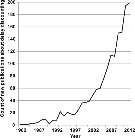
Figure 1: Graph illustrating the rising popularity of temporal
discounting as a research topic over the last twenty years. Results
come from searching on ISI Web of Knowledge with Topic=(temporal
discount*) OR Topic=(delay discount*) NOT Topic=(lobe)
Search language=English Lemmatization=On Refined by: General
Categories=( SOCIAL SCIENCES ), broken down by year.
Despite the growing popularity of research on temporal discounting
(Figure 1), there is relatively little consensus or empirical research
on which methods are best for measuring discounting. Most of the
theoretical and empirical efforts have been directed at testing rival
exponential versus hyperbolic discounting models. The continuously
compounded exponential discount rate (Samuelson, 1937) is calculated
as V = Ae−kD, where V is the present value, A is
the future amount, e is the base of the natural logarithm, D
is the delay in years, and k is the discount rate. This is a normative
model of discounting, which specifies how rational decision makers
ought to evaluate future events, but it has often been employed as a
descriptive model as well. The hyperbolic model (Mazur, 1987) is a
descriptive model, calculated as V = A / (1+kD), where V is the
present value, A is the future amount, D is the delay,1 and k is
the discount rate. Although the hyperbolic and exponential models are
often highly correlated,2 the hyperbolic model often fits the data
somewhat better (e.g., Kirby, 1997; Kirby & Marakovic, 1995; Myerson
& Green, 1995; Rachlin, Raineri, & Cross, 1991). Because most recent
psychological studies of discounting have employed the hyperbolic
model, our further analyses in this paper will focus on this model.
In addition to these two popular discounting metrics, others have been
proposed and tested (for a recent review, see Doyle, 2013). In
contrast, investigations of different experimental procedures for
eliciting discount rates are rare. A comprehensive review paper on
discounting (Frederick, Loewenstein, & O’Donoghue, 2002) noted the
huge variability in discount rates among studies, and hypothesized
that heterogeneity in elicitation methods might be a major cause.
Fifty-two percent of studies reviewed used choice-based
measures, 31% used matching, and 17% used another method.
1.1 Measuring discount rates: Choice versus matching
Choice-based methods often present participants with a series of
binary comparisons and use these to infer an indifference point, which
is then converted into a discount rate. For example, suppose a
participant, presented with a choice between receiving $10
immediately or $11 in one year, chooses the immediate option, and
subsequently, presented with a choice between $10 or $12 in one
year, chooses the future option. This pattern of choices implies that
the participant would be indifferent between $10 today and some
amount between $11 and $12 in one year. For analytic convenience, we
assign their indifference point as the average of the upper and lower
bound, which would be $11.50 in this case. This indifference point
can then be converted into a discount rate using one of the
discounting models discussed above. For example, using the
continuously compounded exponential model, this would yield a discount
rate of 14%. The matching method, in contrast, asks for the exact
indifference point directly. For example, it might ask the participant
what amount “X” would make her indifferent between $10 immediately
and $X in one year.
How do discount rates from these two elicitation methods compare?
Several studies have concluded that matching yields lower discount
rates than choice (Ahlbrecht & Weber, 1997; Manzini, Mariotti, &
Mittone, 2008; Read & Roelofsma, 2003). What are the reasons or
mechanisms for this difference? One hypothesis is that, in choice,
people are motivated to take the earlier reward, and pay relatively
more attention to the delay (rather than the greater magnitude) of the
later reward, whereas the matching methods, which typically ask for a
match on the dollar dimension, focus them on the magnitude of the two
rewards and thus results in a better attentional balance between the
magnitude and delay attributes (Tversky, Sattath, & Slovic,
1988). This attentional hypothesis predicts order effects
(specifically, that the first method will bias attention throughout
the task), but unfortunately neither study investigated task
order,3 so it is difficult to know whether participants’
experience with one method influenced their answers on the other
method. Frederick (2003) compared seven different elicitation methods
(choice, matching, rating, “total”, sequence, “equity”, and
“context”) for saving lives now or in the future. He also found that
matching produced lower discount rates than choice, but again, order
effects were not explored. He speculated that the choice task creates
demand characteristics: offering the choice between different amounts
of immediate and future lives implies that one ought to discount them
to some extent—“otherwise, why would the experimenter be asking the
question” (Frederick, 2003, p. 42). In contrast, the matching method
makes no suggestions as to which amounts are appropriate.
Further evidence that characteristics of offered choice options can
bias discount rates comes from a pair of studies that compared two
variations on a choice-based measure. One version presented repeated
choices that kept the larger-later reward constant with the amounts of
the smaller-sooner reward presented in ascending order, while the
other version employed the same choice pairs, but with the
smaller-sooner amounts presented in descending order. The order of
presentation influenced discount rates, such that participants were
more patient (i.e., exhibited lower discount rates) when answering the
questions in descending order of sooner reward (Robles & Vargas,
2008; Robles, Vargas, & Bejarano, 2009). This suggests that observed
discount rates are at least partly a function of constructed
preference (Stewart, Chater, & Brown, 2006) and “coherent
arbitrariness” (Ariely, Loewenstein, & Prelec, 2003), rather than a
stable individual preference. One explanation offered by Robles and
colleagues is the magnitude effect (i.e., the finding that people are
relatively more patient for large magnitude gains than small magnitude
gains, Thaler, 1981): in the descending condition, participants are
first exposed to largest immediate outcomes, which may predispose them
to choose the future option more readily. In the ascending condition,
participants see the smallest magnitude outcomes first, which may
predispose them to impatience. In other words, the theory is that
participants construct their time preference during the first question
or two, and then carry this preference forward into the rest of the
task, consistent with theories of order effects in constructed choice
such as Query Theory (Weber & Johnson, 2009; Weber et al., 2007).
The question of how choice versus matching influences people’s answers
has also been explored in the context of utility measurement and
public policy (Baron, 1997), with conflicting results. Some studies
suggest that choice methods are more sensitive to quantities
(Fischhoff, Quadrel, Kamlet, Loewenstein, Dawes, Fischbeck, Klepper,
Leland, & Stroh, 1993) and valued attributes (Tversky et al., 1988;
Zakay, 1990), whereas other studies suggest matching is equally or
more sensitive to quantities (Baron & Greene, 1996; McFadden,
1994). Throughout, a key component seems to be joint versus separate
evaluation (Baron & Greene, 1996; Hsee, Loewenstein, Blount, &
Bazerman, 1999): people give more weight to difficult-to-evaluate
attributes in joint evaluation. For example, suppose people find it
easier to evaluate $10 than to evaluate the lives of 2,000 birds. In
single evaluation (“Would you pay $10 to save 2,000 birds?”) people
will put more weight on the financial cost, whereas in joint
evaluation (“Would you choose Program A, that costs $10 and saves
2,000 birds, or Program B, that costs $20 and saves 4,000 birds?”)
people will put more weight on the lives of the birds. Single versus
joint evaluation is often confounded with matching versus choice,
which may explain the conflicting conclusions in the literature.
While these studies show that elicitation method affects responses,
they rarely specify which measure researchers ought to use to
measure discount rates (or which methods to use when). One perspective
on this normative question would argue that because preferences are
constructed, the results from different measures are equally valid
expressions of people’s preferences, and it is therefore impossible to
recommend a best measure. However, when researchers are interested in
predicting and explaining behaviors in real-world contexts, such
behavior provides a metric by which to make a judgment. While several
studies have shown such real-world behavior links for choice-based
techniques, we are not aware of any published studies examining how
well matching-based discount rates predict consequential decisions and
whether they do so better or worse than discount rated inferred from
choice-based methods.4 Another criterion for selecting the “best” measure is
to compare the psychometric properties of each. The ideal measure
would be reliable, with low variance, low demand characteristics, a
good ability to detect inattentive (or dishonest) participants, a
quick completion time, and a straightforward analysis.
Another important question is how well these different elicitation
techniques perform across a broad range of time delays and outcome
dimensions. Most discounting studies have focused only on financial
gains with delays in the range of a few weeks to a few years, but many
consequential real-world intertemporal choices, such as retirement
savings, smoking, or environmental decisions, involve future losses
and much longer time delays. Studying the discounting of complex
outcome sets on long timescales can be logistically difficult in the
lab, if the goal is to make choices consequential: tracking down past
participants in order to send them their “future” payouts is hard
enough one year after a study, but doing so in 50 years may well be
impossible. Truly consequential designs are even trickier when
studying losses, since they require researchers to demand
long-since-endowed money from participants who may not even remember
having participated in the study. Fortunately, hypothetical
delay-discounting questions presented in a laboratory setting do
appear to correlate with real-world measures of impulsivity such as
smoking, overeating, and debt repayment (Chabris et al., 2008; Meier
& Sprenger, 2012; Reimers et al., 2009), suggesting that even
hypothetical outcomes are worth studying.
1.2 Study 1
In Study 1, we compared matching with choice-based methods of
eliciting discount rates for hypothetical financial5 outcomes, in a mixed design. Half the participants
completed matching first followed by choice, while the other half did
the two tasks in the opposite order. This allowed us to analyze the
data both within and between subjects. Within each measurement
technique, delays of the larger-later option varied from 1 year to 50
years. Outcome sign was manipulated between subjects, such that half
the participants considered current versus future gains, while the
other half considered current versus future losses.
Within the choice-based condition, we compared two different
techniques: fixed-sequence titration and a dynamic
multiple-staircase method. The fixed-sequence titration
method presented participants with a pre-set list of choices between a
smaller, sooner amount and a larger, later amount, with all choices
appearing on one page. The multiple-staircase was developed in
psychophysics (Cornsweet, 1962) and attempts to improve on fixed
sequence titration in several ways. First, choice pairs are selected
dynamically, which should reduce the number of questions participants
need to answer (relative to a fixed sequence), yield more precise
estimates, or both. Second, the staircase method approaches
indifference points from above and below, thus reducing anchoring, and
the interleaving of multiple staircases (eliciting several different
indifference points at once, e.g., for different time delays) should
attenuate false consistency, which should reduce demand
characteristics and coherent arbitrariness. Third, we built
consistency-check questions into the multiple-staircase method, which
should enable it to better detect inattention or confusion.
At the end of the survey, we presented participants with a
consequential choice between $100 today or $200 next year, and
randomly paid out two participants for real money. We also asked
participants whether they smoked or not, to get data on a
consequential life choice.
We compared the three elicitation methods on four different criteria:
ability to detect inattentive participants, differences in central
tendency and variability across respondents, model fit, and ability to
predict consequential intertemporal choices. We predicted that the
multiple-staircase method would be best at detecting inattentive
participants, because we designed it partly with this purpose in
mind. We predicted that the choice-based methods would show higher
discount rates than the matching method, due to demand characteristics
(as discussed above, previous research suggest that the choice options
presented to participants implicitly suggest discounting). We also
predicted that the choice-based methods would be easier for
participants to understand and use, based on anecdotal evidence from
our own previous research indicating that participants often have a
hard time understanding the concept of indifference, and have a hard
time picking a number “out of the air”, without any reference or
anchor. Finally, we predicted that the choice-based methods would be
better at predicting the consequential choices, because there is a
natural congruence in using choice to predict choice, and because
previous studies have shown the efficacy of choice-based methods as a
consequential-choice predictor, but none have done so for matching.
1.3 Methods
Five hundred sixteen participants (68% female, mean age=38,
SD=13) were recruited from the virtual lab participant pol of
the Center for Decision Sciences (Columbia University) for a study on
decision making and randomly assigned to an experimental
condition. Participants in the gain condition were given the following
hypothetical scenario:
Imagine the city you live in has a budget surplus that it is planning
to pay out as rebates of $300 for each citizen. The city is
also considering investing the surplus in endowment funds that will
mature at different possible times in the future. The funds
would allow the city to offer rebates of a different amount, to be
paid at different possible times in the future. For the purposes of
answering these questions, please assume that you will not move away
from your current city, even if that is unlikely to be true in
reality.
The full text of all the scenarios can be found in the Supplement
[A]. After reading the scenario, participants indicated their
intertemporal preferences in one of three different ways. In the
matching condition, participants filled in a blank with an amount that
would make them indifferent between $300 immediately and another
amount in the future (see the Supplement [B] for examples of the
questions using each measurement method). Participants answered
questions about three different delays: one year, ten years, and 50
years. Although some participants might expect to be dead in 50 years,
the scenario described future gains that would benefit everyone in
their city, so it was hoped that those future gains would still have
meaning to participants. In the titration condition, participants made
a series of choices between immediate and future amounts, at each
delay. Because the same set of choice options was presented for each
delay (see Supplement [B] for the list of options), the choice set
offered a wide range of values, to simultaneously ensure that time
delay and choice options were not confounded and allow for high
discount rates at long delays. The order of the future amounts was
balanced between participants, such that half answered lists with the
amounts of the larger-later option going from low to high (as in the
Supplement [B]), and others were presented with amounts going from
high to low.
In the multiple-staircase condition, participants also made a series
of choices between immediate and future amounts. Unlike the simple
titration method, these amounts were selected dynamically, funneling
in on the participant’s indifference point. Choices were presented
one at a time (unlike titration, which presented all choices on one
screen). Also unlike titration, the questions from the three delays
were interleaved in a random sequence. The complete multiple-staircase
method is described in detail in the Supplement [C].
In all conditions progress in the different tasks of the questionnaire
was indicated with a progress bar, and participants could refer back
to the scenario as they answered the questions. After completing the
intertemporal choice task, participants were asked “What things did
you think about as you answered the previous questions? Please give a
brief summary of your thoughts.” This allowed us to collect
some qualitative data on the processes participants recalled using
while responding to the questions.
Next, participants answered the same intertemporal choice scenario
using a different measurement method. Those who initially were given a
choice-based measure (titration or multiple-staircase) subsequently
completed a matching measure, while those who began with matching then
completed a choice-based measure. In other words, all participants
completed a matching measure, either before or after completing one of
the two choice-based measures. Subsequently, participants were given
an attention check, very similar to the Instructional Manipulation
Check (Oppenheimer, Meyvis, & Davidenko, 2009) that ascertained
whether participants were reading instructions.
After that, participants read an environmental discounting scenario
(order of financial vs. environmental scenario was not
counterbalanced), the full text of which can be found in the
Supplement [A]. We do not discuss the results from this scenario
because of possible conceptual confusion in the questions themselves,
and other problems.
Next, participants provided demographic information, including a
question about whether they smoked. Finally, participants completed a
consequential measure of intertemporal choice, in which they chose
between receiving $100 immediately or $200 in one year (note that
participants in the loss condition still chose between two gains in
this case, due to the fact that it would have be difficult to execute
losses for real money). Participants were informed that two people
would be randomly selected and have their choices paid out for real
money, and this indeed happened.
1.4 Results and discussion
1.4.1 Detecting inattentive participants
In most psychology research, and especially in online research, a
portion of respondents does not pay much attention or does not respond
carefully. It is helpful, therefore, if measurement methods can detect
these participants. The multiple-staircase method had two built-in
check questions (described in the Supplement [C]) to detect such
participants. The titration method can also detect inattention in some
cases, by looking for instances of switching back and forth, or
switching perversely. For example, if a participant preferred $475 in
one year over $300 today, but preferred $300 today over $900 in one
year, this inconsistency would be a sign of inattention. Titration
cannot, however, differentiate between “good” participants and those
who learn what a “good” pattern of choices looks like and reproduce
such a pattern for later questions, without carefully considering each
subsequent question individually. It is nearly impossible for a single
matching measure to detect inattention, but with multiple measures
presented at different time points, matching may identify those
participants who show a non-monotonic effect of time. For example, if
the one-year indifference point (with respect to $300 immediately) is
$5,000, the ten-year indifference point is $600, and the 50-year
indifference point is $50,000, this inconsistency might be evidence
of inattention.
As described above, each participant also completed another attention
check, very similar to the Instructional Manipulation Check (IMC,
Oppenheimer et al., 2009). As this measure has been empirically shown
to be effective for detecting inattentive participants, we compared
the ability of each measurement method to predict IMC status.
Correlations between the IMC and each measure’s test of attention
revealed that while neither matching, r (253) = .06,
p > .1, nor titration, r (124) = .04,
p > .1 were able to detect inattentive
participants, the multiple-staircase method had modest success,
r (132) = .21, p < .05. Overall, then, no
method was particularly effective at detecting inattentive
participants, but the multiple-staircase method was apparently
superior to the other two. It was not surprising that
multiple-staircase performed better in this regard, given that it was
designed partly with this purpose in mind, but it was
surprising that titration did not outperform matching in this regard,
given that titration gave participants ten times as many questions,
and as such provided more opportunities to detect inattention.
For all of the following analyses, we compared only those participants
who were paying attention and reading instructions, because the
indifference points of participants who did not read the scenario are
of questionable validity. Also, it is fairly common in research on
discounting (and online research in particular) to screen out
inattentive participants (see Ahlbrecht & Weber, 1997; Benzion,
Rapoport, & Yagil, 1989; Shelley, 1993). Therefore, we excluded
those participants who failed the IMC, leaving 316 participants (61%
of the original sample) for further analysis. The rate of inattentive
participants did not vary as a function of measurement condition,
χ 2 (2,N=516)=0.8,
p=.67. (For analyses with all participants included, see the
Supplement [D]. Overall, the results are quite similar, but variance
and outliers are increased.)
1.4.2 Differences in central tendency and spread
Choice indifference points were determined for each scenario,
participant, and time delay as follows: in matching, the number given
by participants was used directly. For titration, the average of the
values around the switch point was used. For example, if a participant
preferred $300 immediately over $475 in ten years, but preferred
$900 in ten years over $300 immediately, the participant was judged
to be indifferent between $300 immediately and $687.50 in ten
years. For multiple-staircase, the average of the established upper
bound and lower bound was used, in a similar manner to
titration. These choice indifference points were then converted to
discount rates, using the hyperbolic model described in the
introduction.
Table 1: Means, standard deviations, medians, and interquartile ranges
(IQRs) for three methods of eliciting hyperbolic discount rates
(matching, multiple-staircase, and titration) for financial gains
and losses.
Financial outcome
Hyperbolic discount rate
Mean
SD
Median
IQR
Matching, gain
2.51
8.59
0.75
1.05
M-stairs, gain
6.03
16.01
2.55
2.04
Titration, gain
10.27
34.43
1.59
3.02
Matching, loss
0.53
1.47
0.15
0.41
M-stairs, loss
1.29
2.92
0.29
0.54
Titration, loss
3.71
14.29
0.15
0.52
Because order effects were observed (which we describe below), the
majority of the analyses to follow will focus on the first measurement
method that participants completed. This leaves n=154 in the
matching condition, n=82 in the titration condition, and
n=80 in the multiple-staircase condition.6 Discount
rates for financial outcomes in each condition are summarized in Table
1. Because skew and outliers were sometimes pronounced, this table
lists median and interquartile range in addition to mean and standard
deviation.
As shown in Table 1 and consistent with prior results (Ahlbrecht &
Weber, 1997; Read & Roelofsma, 2003), financial discount rates
measured with the choice-based methods (titration and
multiple-staircase) were generally higher than discount rates measured
with matching, and this was particularly true for gains. A
Kruskal-Wallis non-parametric ANOVA of the financial gain data, χ
2 (2, n = 148) = 26.8, p
< .001, and of the loss data, χ 2
(2, n = 168) = 6.8, p = .03, confirmed a significant
effect of elicitation method on discount rates.
We hypothesized that these differences in discount rates were partly a
function of anchoring or demand characteristics. In other words, the
extreme options sometimes presented to participants (such as a choice
between $300 today and $85,000 in one year) may have suggested that
these were reasonable choices, and so encouraged higher discount
rates. Consistent with this explanation, an earlier study from our
lab (Hardisty & Weber, 2009, Study 1)—with a different sample
recruited from the same participant population and using titration for
financial outcomes—presented participants with a much smaller range
of options ($250 today vs. $230 to $410 in one year) and yielded
much lower median discount rates: 0.28 for gains, and 0.04 for losses,
compared with medians of 1.59 for gains and 0.14 for losses in the
present study. It seems, then, the range of options presented to
participants affected their discount rates by suggesting reasonable
options as well as by restricting what participants could or could not
actually express (for example, an extremely impatient person might
prefer $250 today over $1,000 next year, but if the maximum choice
pair is $250 today vs. $410 in one year, the experimenter would
never know). We also tested for the influence of the options presented
to participants by comparing the two orderings, descending and
ascending. As summarized in Figure 2, this ordering manipulation did
indeed affect responses. Consistent with previous studies on order
effects in titration (Robles & Vargas, 2008; Robles et al., 2009),
participants exhibited lower discount rates in the descending order
condition, possibly as a result of the magnitude effect. Losses show
the opposite order effect (by “ascending order” for losses, we mean
ascending in absolute value), which is consistent with the reverse
magnitude effect recently found with losses (Hardisty, Appelt, &
Weber, 2012): people considering larger losses are more likely to want
to postpone losses.
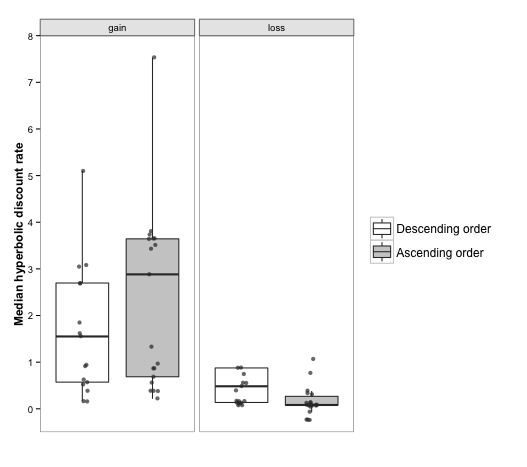
Figure 2: Boxplots of median hyperbolic discount rates for financial gains and
losses as measured with titration, broken down by the order in which
future amounts were presented. The crossbar of each box represents
the median; the bottom and top edges of the box mark the first and
third quartiles, respectively, and the whiskers each extend to the
last outlier that is less than 1.5 IQRs beyond each edge of the
box. Each dot represents one data point. Points are jittered
horizontally, but not vertically: the vertical position of each
point represents one participant’s hyperbolic discount rate. Nine
data points lie outside the range of this figure: 3 in the gain
condition (1 descending; 2 ascending) and 6 in the loss condition (5
descending; 1 ascending).
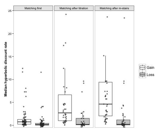
Figure 3: Boxplots of median hyperbolic discount rates for financial
gains and losses as measured with matching, broken down by whether
participants did the matching task before or after one of the
choice-based measurement methods. The crossbar of each box
represents the median; the bottom and top edges of the box mark
the first and third quartiles, respectively, and the whiskers each
extend to the last outlier that is less than 1.5 IQRs beyond each
edge of the box. Each dot represents one data point. Points are
jittered horizontally, but not vertically: the vertical position
of each point represents one participant’s hyperbolic discount
rate. Thirteen data points lie outside the range of this figure: 1
for matching first, and 6 each in the conditions where matching
followed a choice method.
A Mann-Whitney U test comparing the descending and ascending
orderings for losses was significant, W = 363, n =
43, p < .01, showing greater discounting in the
descending order. A similar test comparing the two orderings for gains
was not significant, W = 141, n = 38, p =
.28, (the sample size was somewhat small here, with only 17
participants in the ascending condition, and 21 in the descending) but
was in the predicted direction, with higher discount rates in the
ascending order condition.
While discount rates were generally much higher when using the
choice-based methods, we believe that this difference was due to the
large range of options that we presented to participants, and it would
be possible to obtain the opposite pattern of results if a smaller
range were used. For example, if the maximally different choice pair
were $300 today vs. $400 in the future (rather than $85,000, as we
used), this presentation would result in lower discount rates, both
through demand characteristics (suggesting that lower discount rates
are reasonable) and by restricting the range of possible
answers. Further evidence for this explanation comes from a
within-subject analysis comparing the different methods: although all
participants completed a matching measure, some did so before a choice
method, and some did so after a choice method. Comparing these
participants reveals a significant effect of order, as seen in Figure
3, such that discount rates assessed by matching were larger when they
followed a choice-based elicitation method.
A Mann-Whitney U test confirmed that participants gave
different answers to the matching questions depending on whether they
completed a choice based measure first or second, both for gains,
W = 4373, n = 147, p < .001, and
losses, W = 4211, n = 166, p =
.02. Furthermore, participants’ answers to the matching and
choice-based questions were strongly correlated, Spearman’s
r(269) = .52, p < .001.
Just as the mean and median discount rates yielded by the choice-based
methods were higher than those from the matching method, so too was
the spread of the distributions from the choice-based methods
larger. The interquartile range (IQR) from the matching method for
gains was 1.1, compared with 2.0 from multiple-staircase and 3.0 from
titration. Similarly, the IQR for matching losses was only 0.41,
compared with 0.54 from multiple staircase and 0.52 from titration. It
is likely that the same factors that led to the higher medians in the
choice-based methods also produced the greater IQR.
Overall, then, we have three pieces of evidence suggesting that the
options presented to participants in the choice-based methods affected
discount rates: (1) discount rates were higher when using the
choice-based methods, (2) ordering of choice pairs (ascending or
descending) in the titration condition affected discount rates, and
(3) discount rates first elicited with choice methods went on to
influence later responses elicited with matching. While matching has
the advantage of not providing any anchors or suggestions to
participants, it is nonetheless still quite susceptible to influence
from other sources. This is not a particularly novel finding, as
theories and findings of constructed preference (Johnson, Haubl, &
Keinan, 2007; Stewart et al., 2006; Weber et al., 2007) and coherent
arbitrariness (Ariely et al., 2003) are plentiful. However, it has not
received as much attention in intertemporal choice as in other areas
(particularly risk preference). Many differences in discount rates
between studies may be explained by differences in the amount and
order of options that experimenters presented to participants.
1.4.3 Differences in model fit
Table 2: Average fit (r2) of the hyperbolic model to
participants’ indifference points as measured via measured via
matching, multiple-staircase, or titration, in Study 1.
Sign
Measure
Gain
Loss
Matching
.95
.90
Titration
.89
.71
Staircase
.94
.83
Considering that the hyperbolic model is currently the dominant
descriptive model of discounting, a measurement method may be more
desirable if it conforms to this model more closely. Therefore, we fit
k values (using least squares) separately for each participant, and
calculated the average r2 of each
method, as summarized in Table 2. Matching produced the best fit for
both gains and losses, suggesting that the results from matching are
the most consistent with the hyperbolic model. One possible reason for
the superior fit of matching is that it provides exact indifference
points, whereas the choice methods merely provide boundaries on
indifference points.
1.4.4 Predicting consequential choices
Table 3: Non-parametric correlations (Spearman’s rho) between
hypothetical discount rates elicited in different ways and
consequential intertemporal choices. The † symbol
indicates p <.1 two-tailed, * indicates p <.05,
and ** indicates p <.01.
Sign
Elicitation method
Choosing a $100 gain now over $200 in one year
Smoking
Gain
Matching
.07
-.04
M-stairs
.32*
.40**
Titration
.68**
.00
Loss
Matching
.16
.15
M-stairs
.28†
.07
Titration
.26†
.41**
Researchers are often interested in discount rates because they would
like to better understand the real, consequential choices that people
make. We therefore compared the ability of discount rates elicited in
different ways for the hypothetical scenarios to predict two
consequential choices. First, we used the 1-year hyperbolic discount
rate7 to predict whether participants chose to
receive $100 today or $200 in one year in the final consequential
choice they made as part of our study. (Overall, 25% of participants
chose the immediate $100.) As seen in Table 3, the correlations were
always positive, meaning that participants with higher assessed
discount rates were more likely to choose the immediate $100. The
correlations from the choice based measures were generally higher, but
the only significant difference between the correlations was that
titration outperformed both matching (p<.001) and
multiple-staircase (p=.04). The generally stronger
performance of the choice-based methods is consistent with the method
compatibility principle (Weber & Johnson, 2008): predicting a choice
will be more accurate with a choice-based measure than a
fill-in-the-blank measure.
Second, we looked at the ability of these 1-year discount rates to
predict a real-life choice: whether each participant was a smoker or
not. The prediction is that people who discount future financial
outcomes may also discount their future health, and so be more likely
to smoke (Bickel, Odum, & Madden, 1999). As seen in Table 3, the
choice-based methods were sometimes able to predict this (with higher
discount rates correlating with smoking), while the matching method
was not. The multiple-staircase method was significantly
(p=.02 and p=.08) better at predicting smoking rates
with discount rates for gains, while titration was directionally
better at predicting using discount rates for losses (p=.14
and p=.11). We don’t have a good explanation for this
difference, other than random fluctuations. However, the overall trend
was that choice methods yielded greater predictive power than
matching. This may stem from the fact that participants found it
easier to understand and respond to the choice-based measures of
discounting and thus had less error in responding.
2 Study 2
These results suggest that researchers interested in predicting
consequential intertemporal choices should employ choice-based
methods. However, the results are a bit thin and
inconsistent. Therefore, in Study 2, we included measures of eighteen
real-world behaviors (in addition to the $100 vs. $200
consequential choice) that have previously been found to correlate
with discount rates (Chabris et al., 2008; Reimers et al., 2009),
allowing us to compare the measures more rigorously in this regard. A
second shortcoming of Study 1 is that a large proportion of
participants gave inattentive or irrational answers and had to be
excluded from the data set. We addressed this in Study 2 by recruiting
a more conscientious group of participants and building checks into
each measure that prevent participants from giving non-monotonic or
perverse answers. A third weakness of Study 1 is that our complex
multiple-staircase method did not perform well, possibly because
participants found it difficult to use. Therefore, in Study 2, we
tested a simpler dynamic choice method.
2.1 Methods
316 U.S. residents with at least a 97% prior approval rate were
recruited from Amazon Mechanical Turk for a study on decision making
and paid a flat rate of $1. Participants (59% female, mean age=34,
SD=11.9) were randomly assigned to one of three conditions:
matching, titration, or single-staircase (described
below). Participants answered questions about immediate versus future
gains and losses (in counterbalanced order) at delays of 6 months, 1
year, and 10 years.8
In the matching condition, participants saw this instruction:
Imagine you could choose between receiving [paying] $300 immediately, or another amount 6 months [1 year
| 10 years] from now. How much would the future amount need to be to make it as attractive [unattractive] as
receiving [paying] $300 immediately?
Please fill in the dollar amount that would make the following options equally attractive [unattractive]:
A. Receive [Lose] $300 immediately.
B. Receive [Lose] $____
After participants entered a value for each delay, an automated script
checked whether the amounts increased or decreased in a monotonic
fashion. If not, the participant was given the instruction, “Your
answers were inconsistent over time. Please try this scale again, and
be more careful as you answer”, and was forced to go back and enter
new values. Note that participants were allowed to show
negative discounting (for example, indicating that losing $300 today
would be equivalent to losing $290 in six months, $280 in one year,
and $120 in ten years). Such a pattern of responding has previously
been observed in studies of discounting (Hardisty et al., 2012;
Hardisty & Weber, 2009) and can be considered a rational way to avoid
dread (Harris, 2010).
In the titration condition, participants saw this instruction:
“Imagine you could choose between receiving [paying] $300
immediately, or another amount 6 months [1 year | 10 years]
from now. Please indicate which option you would choose in each
case:” Participants then made a series of 10 choices at each delay
(the complete list can be found in the Supplement [E]), such as
“Receive $300 immediately OR Receive $350 in 6 months”. The future
amounts ranged from $250 to $10,000. As in Study 1, all questions
for a given sign were presented on one page. In other words, one page
had 30 questions about immediate versus future gains, and another page
(in counterbalanced order) had 30 questions about immediate versus
future losses. Participants’ answers were automatically checked for
nonmonotonicity or perverse switching (such as choosing to receive
$350 in one year over $300 immediately, and then choosing $300
immediately over $400 in one year), and participants were forced to
go back and redo their answers if they violated either of these
principles.
In the single-staircase condition, participants answered one question
per page, and each choice option was dynamically generated, using
bisection. The upper and lower ends of each staircase were set to
$200 and $15,000 (the maximum and minimum possible implied
indifference points using the titration scale). The first question cut
the possible range in half, and thus was always “Receive $300
immediately OR Receive $7,600 in 6 months.” The next question then
cut the range in half again, in the direction indicated by the prior
choice. For example, if the participant chose the future option, the
second question would be “Receive $300 immediately OR Receive
$3,900 in 6 months.” Ten questions were asked in this way at each
time delay.
Subsequently, all participants answered a number of demographic
questions (mostly drawn from Chabris et al., 2008; Reimers et al.,
2009): gender, age, education, relevant college courses, ethnicity,
political affiliation, height, weight, exercise, dieting, healthy
eating, dental checkups, flossing, prescription following, tobacco
use, alcohol consumption, cannabis use, other illegal drug use, age of
first sexual intercourse, recent relationship infidelity, annual
household income, number of credit cards, credit-card late fees,
carrying a credit card balance, savings, gambling, wealth relative to
friends, wealth relative to family, and available financial
resources. Finally, participants made a consequential choice between a
$100 Amazon gift certificate today or a $200 gift certificate in one
year, and one participant was randomly selected and paid out for real
money. The full text of all Study 2 materials can be found in the
Supplement [E].9
2.2 Results and Discussion
Data were excluded from 5 participants with duplicate IP addresses, 13
participants who did not finish the study, and 22 participants who
failed an attention check (similar to the attention check used by
Oppenheimer et al., 2009), leaving 276 for further analysis. Although
the rate of attention check failure did not vary by condition,
χ 2 (2, N=311)=2.5,
p=.29, the number of participants that failed to complete the
study did: 10% of participants in the staircase condition
dropped out, compared with 3% in the titration condition and 0% in
the matching condition, χ 2 (2,
N=311)=13.01, p<.01. This difference in
completion rates may have been caused by the fact that participants in
the staircase condition were more likely to fail the monotonicity
checks (and be forced to go back and complete the measure again). When
considering immediate versus future gains, 0% of participants in the
matching condition initially gave answers that were non-monotonic over
time, compared with 2% in the titration condition (with the titration
condition including both nonmonotonic answers and perverse switching),
and 13% in the staircase condition, a significant difference with a
Chi-square test, χ 2 (2, N=276) =
18.3, p < .01. Follow-up pairwise comparisons
showed that while the staircase method showed more nonmonotonicities
than each of the other two methods, matching and titration did not
differ from each other. Similarly, when comparing immediate versus
future losses, 2% of participants in the matching condition initially
gave answers that were non-monotonic over time, compared with 4% in
the titration condition, and 10% in the staircase condition, a
significant difference, χ 2 (2, N=276)
= 6.3, p < .05. In follow-up pairwise comparisons,
a greater proportion of participants showed nonmonotonicities when
using staircase than when using matching, p = .05, but no
other comparisons were significant. Across conditions, only 76% of
participants who failed a monotonicity check finished the study,
compared with 99% of those who passed all monotonicity checks, a
significant difference in proportions, z=3.2
p<.01.
Another possible reason dropout rates were higher in the staircase
condition is that the study was significantly longer: participants
spent a median of 10.6 minutes completing the survey in the staircase
condition, compared with 7.8 in the titration condition and 6.3 in the
matching condition, a significant difference with a Kruskal-Wallis
test, χ 2 (2, N=276) = 70.2, p
< .01. Pairwise tests were all significant, ps
< .01.
2.2.1 Differences in central tendency and spread
Table 4: Means, standard deviations, medians, and interquartile ranges
(IQRs) for three methods (matching, dynamic staircase, and
titration) of eliciting hyperbolic discount rates for financial
gains and losses.
Measure
Mean
SD
Median
IQR
Matching, gain
10.66
60.58
1.74
2.72
Titration, gain
1.34
2.05
0.82
1.16
Staircase, gain
2.26
5.54
0.81
2.38
Matching, loss
1.21
2.19
0.63
1.11
Titration, loss
0.47
0.59
0.26
0.55
Staircase, loss
1.30
4.51
0.34
1.06
Hyperbolic discount rates were calculated using the same method as for
Study 1. The distributions of discount rates were generally quite
skewed, so we will focus our analysis on non-parametric measures and
tests. As can be seen in Table 4, the matching method produced larger,
more variable discount rates than the two choice based methods.
Kruskal-Wallis tests for gains, χ 2 (2,
n = 276) = 31.0, p < .001, and losses,
χ 2 (2, n = 276) = 9.1, p =
.01, confirmed that median discount rates varied as a function of
measurement method. Follow-up pairwise comparisons confirmed that
while matching was higher than each of the choice based methods, the
choice-based methods did not differ significantly from each other.
This pattern of discount rates is opposite of that observed in Study 1
(where discount rates from matching were lowest, and the spread from
matching was smallest). The difference between the Study 1 and 2
results can probably be attributed to the fact the range of choice
options in the titration and staircase conditions was much lower in
Study 2 (maximum future payout = $10,000) than in Study 1 (maximum
future payout = $85,000). This reinforces the importance of not only
the method that researchers use (ie, choice vs matching), but the
specific details of that method (ie, the range and order of the choice
options).
2.2.2 Differences in model fit
Table 5: Average fit (r2) of the hyperbolic model to participants’ indifference
points as measured via measured via matching, multiple-staircase, or titration, in Study 2.
Sign
Measure
Gain
Loss
Matching
.98
.90
Titration
.92
.84
Staircase
.88
.78
As in Study 1, we computed how well the results of each measure fit
the hyperbolic model. As seen in Table 5, matching showed the best
fit, replicating the results of Study 1.
2.2.3 Predicting consequential choices
Table 6: Non-parametric correlations (Spearman’s
rho) between consequential outcomes and discount rates for gains
and losses, measured via matching, titration, or dynamic
staircase, in Study 2.
Outcome
Matching
Titration
Staircase
Gains
Losses
Gains
Losses
Gains
Losses
Tobacco
.12
.02
.23*
.08
.18†
.12
Chose future $200§
.42**
.21*
.38**
.23*
.37**
.28**
Financial resources§
.37**
.17
.22*
.28**
.08
.29**
Exercise§
-.17
-.07
.22*
.29**
.08
.13
Diet§
.13
-.10
.01
.03
.17
.16
Healthy eating§
.11
.10
.02
.11
.24*
.16
Overeating
.06
-.03
.13
.11
.10
.05
Dental checkups§
.01
.12
.11
.21*
.28**
.22*
Flossing§
.02
.08
.19†
.25**
.12
.15
Follow prescriptions§
.17
.20*
.11
.10
-.08
.09
Age of first sex
.21*
.04
.17
.05
.07
-.15
Recent infidelity
.02
.05
.18†
.10
.24*
.19†
BMI
-.14
-.12
.13
.04
.14
.09
Credit late fees
.33**
.24†
.10
.31**
.30*
.52**
Credit paid in full§
.12
.18
.25*
.38**
.52**
.56**
Savings§
.06
.18†
.25**
.35**
.22*
.23*
Gambling
-.01
.03
.18†
.12
.21*
.15
Wealth / friends§
.14
.18†
.21*
.15
.11
.22*
Wealth / family§
.09
.15
.26**
.13
.10
.20†
Avg. correlation
.11
.09
.18
.17
.18
.19
§ this item was reverse scored; **
p<.01; * p<.05; †
p<.01.
Finally, and perhaps most importantly, we compared the correlations of
each measure with real-world outcomes. We reverse scored several items
(indicated in Table 6) so that positive values indicate a correlation
in the predicted direction. As can be seen in Table 6, the
choice-based measures generally outperformed matching, with
correlations around .18 (compared with .10 on average for
matching). Replicating Study 1, the choice-based measures
significantly predicted tobacco use, while matching did not. Unlike
Study 1, both matching and the choice-based measures significantly
predicted the consequential choice between $100 now and $200 in one
year10. This improvement might be attributed to the fact that in
Study 2 we used a subject population (MTurk workers) that may be more
experienced with survey questions and more careful than our previous
subject population. It is also notable that credit-card behavior and
savings behavior were generally well predicted by discount rates,
which makes sense because these are clean examples of real-life
choices between gaining or losing money now or in the future.
3 Conclusions
Choice-based measures of discounting are a double-edged sword, to be
used carefully. On the one hand, they generally outperform matching at
predicting consequential intertemporal choices. On the other hand, the
options (and order of options) that researchers use will influence
participants’ answers, so experimental design and interpretation must
be done with care. Matching introduces less experimenter bias, is
faster to implement, and produces a better fit with the hyperbolic
model of discounting. Differences in discount rates observed between
studies may be partly attributed to differences in elicitation
technique, consistent with long-established research on risky choice
that has come to the same conclusion (Lichtenstein & Slovic, 1971;
Tversky et al., 1988). Across all methods, we found strong evidence
for the sign effect (gains being discounted more than losses),
replicating previous research (Frederick et al., 2002; Hardisty &
Weber, 2009; Thaler, 1981). In other words, participants’ desire to
have gains immediately was stronger than their desire to postpone
losses.
In Study 1, the choice-based measures presented participants with a
large range of outcomes, and therefore yielded higher
discount rates than the matching method, whereas in Study 2 the range
of outcomes was more restricted and thus the choice-based measures
yielded lower discount rates. We agree with Frederick (2003)
that the range of options participants see implicitly suggests
appropriate discount rates. Consistent with this, when doing
within-subject analyses, we found strong order effects; participants
gave very different responses to the matching questions depending on
whether they completed them before or after a choice-based
method. Therefore, future research on methods should be careful to
counterbalance and investigate order effects.
Another disadvantage of choice-based methods is that they take longer
for participants to complete (and longer for the experimenter to
analyze). In our studies, the matching method was about 1.5 minutes
faster than titration (and 4.3 minutes faster than the staircase
method). Thus may seem trivial, but if participants are financially
compensated for their time, matching is cheaper to run, and if the
research budget is limited, matching therefore allows for larger
sample sizes or more studies.
In comparison with the standard, fixed-sequence titration method, we
did not find compelling advantages for the complex multiple-staircase
method we developed in Study 1, nor for the simple dynamic staircase
method we tested in Study 2. This is consistent with another recent
study on dynamic versus fixed-sequence choice, which also found no
mean differences (Rodzon, Berry, & Odum, 2011). In some ways, it is
disappointing that our attempts to improve measurement were
unsuccessful. However, the good news is that the simple titration
measure, which is much more convenient to implement, remains a useful
method.
While we focused on choice and matching elicitation methods because
these have been most commonly used in the literature, it should be
noted that many other techniques have recently been tested and
compared, including intertemporal allocation, evaluations of
sequences, intertemporal auctions, and evaluation of amounts versus
interest rates (Frederick & Loewenstein, 2008; Guyse & Simon, 2011;
Manzini et al., 2008; Olivola & Wang, 2011; Read, Frederick, &
Scholten, 2012). All of these investigations have found differences in
discount rates based on the elicitation methods. Taken together with
our results, this strongly suggests that intertemporal preferences are
partly constructed, based on the manner in which they are elicited. At
the same time, the correlations between lab measured discount rates
and real-world intertemporal choices such as smoking establish that
intertemporal preferences are also partly a stable individual
difference that is manifested across diverse contexts.
In terms of best practices for studying temporal discounting, our
recommendation depends on the goal of the research project. If the
goal is to predict real-world behavior and outcomes, choice-based
methods should be used, whereas if the goal is to minimize
experimental demand effects, secure a good model fit, or quickly
obtain an exact indifference point, matching should be used.
References
Ahlbrecht, M., & Weber, M. (1997). An empirical study on
intertemporal decision making under risk. Management Science,
43, 813–826. http://dx.doi.org/10.1287/mnsc.43.6.813
Ariely, D., Loewenstein, G., & Prelec, D. (2003). “Coherent
arbitrariness”: Stable demand curves without stable
preferences. The Quarterly Journal of Economics, 118,
73–105. http://dx.doi.org/10.1162/00335530360535153
Baron, J. (1997). Biases in the quantitative measurement of values for
public decisions. Psychological Bulletin, 122, 72–88.
Baron, J., & Greene, J. (1996). Determinants of insensitivity to
quantity in valuation of public goods: Contribution, warm glow, budget
constraints, availability, and prominence. Journal of
Experimental Psychology: Applied, 2, 107–125.
Benzion, U., Rapoport, A., & Yagil, J. (1989). Discount rates
inferred from decisions: An experimental study. Management
Science, 35, 270–284. http://dx.doi.org/10.1287/mnsc.35.3.270
Bickel, W. K., Odum, A. L., & Madden, G. J. (1999). Impulsivity and
cigarette smoking: Delay discounting in current, never-, and
ex-smokers. Psychopharmacology, 146,
447–454. http://dx.doi.org/10.1007/PL00005490
Chabris, C. F., Laibson, D., Morris, C. L., Schuldt, J. P., &
Taubinsky, D. (2008). Individual laboratory-measured discount rates
predict field behavior. Journal of Risk and Uncertainty,
37. http://dx.doi.org/10.1007/s11166-008-9053-x
Cornsweet, T. N. (1962). The staircase method in
psychophysics. American Journal of Psychology, 75, 485–491.
Daly, M., Harmon, C. P., & Delaney, L. (2009). Psychological and
biological foundations of time preference. Journal of the
European Economic Association, 7, 659–669.
Doyle, J. R. (2013). Survey of time preference, delay discounting
models. Judgment and Decision Making, 8, 116–135.
Doyle, J. R., Chen, C. H., & Savani, K. (2011). New designs for
research in delay discounting. Judgment and Decision Making,
6, 759–770.
Fischhoff, B., Quadrel, M. J., Kamlet, M., Loewenstein, G., Dawes, R.,
Fischbeck, P., Klepper, S., Leland, J., & Stroh, P. (1993). Embedding
effects: Stimulus representation and response mode. Journal of
Risk and Uncertainty, 6, 211–234.
Frederick, S. (2003). Measuring intergenerational time preference: Are
future lives valued less? Journal of Risk & Uncertainty, 26,
39–53. http://dx.doi.org/10.1023/A:1022298223127
Frederick, S., & Loewenstein, G. (2008). Conflicting motives in
evaluations of sequences. Journal of Risk & Uncertainty, 37,
221–235. http://dx.doi.org/10.1007/s11166-008-9051-z
Frederick, S., Loewenstein, G., & O’Donoghue, T. (2002). Time
discounting and time preference: A critical review. Journal
of Economic Literature, 40, 351–401. http://dx.doi.org/10.1257/002205102320161311
Guyse, J. L., & Simon, J. (2011). Consistency among elicitation
techniques for intertemporal choice: A within-subjects investigation
of the anomalies. Decision Analysis, 8, 233–246.
Hardisty, D. J., Appelt, K. C., & Weber, E. U. (2012). Good or bad,
we want it now: Fixed-cost present bias for gains and losses explains
magnitude asymmetries in intertemporal choice. Journal of
Behavioral Decision Making, in press.
Hardisty, D. J., & Weber, E. U. (2009). Discounting future green:
Money versus the environment. Journal of Experimental
Psychology: General, 138, 329–340. http://dx.doi.org/10.1037/a0016433
Harris, C. R. (2010). Feelings of dread and intertemporal
choice. Journal of Behavioral Decision
Making. http://dx.doi.org/10.1002/bdm.709
Hsee, C., Loewenstein, G., Blount, S., & Bazerman,
M. (1999). Preference reversals between joint and separate evaluations
of options: A review and theoretical analysis. Psychological
Bulletin, 125, 06–14.
Johnson, E. J., Haubl, G., & Keinan, A. (2007). Aspects of endowment:
A query theory of value. Journal of Experimental Psychology:
Learning, Memory, and Cognition, 33,
461–474. http://dx.doi.org/10.1037/0278-7393.33.3.461
Kirby, K. N. (1997). Bidding on the future: Evidence against normative
discounting of delayed rewards. Journal of Experimental
Psychology: General, 126, 54–70. http://dx.doi.org/10.1037//0096-3445.126.1.54
Kirby, K. N., & Marakovic, N. N. (1995). Modeling myopic decisions:
Evidence for hyperbolic delay-discounting with subjects and
amounts. Organizational Behavior and Human Decision Processes,
64, 22–30. http://dx.doi.org/10.1006/obhd.1995.1086
Lichtenstein, S., & Slovic, P. (1971). Reversals of preference
between bids and choices in gambling decisions. Journal of
Experimental Psychology, 89, 46–55. http://dx.doi.org/10.1037/h0031207
Manzini, P., Mariotti, M., & Mittone, L. (2008). The elicitation of
time preferences. Working paper.
Mazur, J. E. (1987). An adjusting procedure for studying delayed
reinforcement. In M. L. Commons, J. E. Mazure, J. A. Nevin &
H. Rachlin (Eds.), Quantitative analyses of behavior:
Vol. 5. The effect of delay and intervening events on reinforcement
value (pp. 55–73). Hillsdale, NJ: Erlbaum.
McFadden, D. (1994). Contingent valuation and social
choice. American Journal of Agrigultural Economics, 76,
689–708.
Meier, S., & Sprenger, C. (2010). Present-biased preferences and
credit card borrowing. American Economic Journal: Applied
Economics, 2, 193–210. http://dx.doi.org/10.1257/app.2.1.193
Meier, S., & Sprenger, C. (2012). Time discounting predicts
creditworthiness. Psychological Science, 23, 56–58.
Oppenheimer, D. M., Meyvis, T., & Davidenko, N. (2009). Instructional
manipulation checks: Detecting satisficing to increase statistical
power. Journal of Experimental Social Psychology, 45,
867–872. http://dx.doi.org/10.1016/j.jesp.2009.03.009
Rachlin, H., Raineri, A., & Cross, D. (1991). Subjective probability
and delay. Journal of the Experimental Analysis of Behavior,
55, 233–244. http://dx.doi.org/10.1901/jeab.1991.55-233
Read, D., Frederick, S., & Scholten, M. (2012). Drift: An analysis of
outcome framing in intertemporal choice. Journal of
Experimental Psychology: Learning, Memory, and Cognition, in press.
Read, D., & Roelofsma, P. (2003). Subadditive versus hyperbolic
discounting: A comparison of choice and matching.
Organizational Behavior & Human Decision Processes, 91,
140–153. http://dx.doi.org/10.1016/S0749-5978(03)00060-8
Reimers, S., Maylor, E. A., Stewart, N., & Chater,
N. (2009). Associations between a one-shot delay discounting measure
and age, income education and real-world impulsive
behavior. Personality and Individual Differences, 47,
973–978. http://dx.doi.org/10.1016/j.paid.2009.07.026
Robles, E., & Vargas, P. A. (2008). Parameters of delay discounting
assessment: Number of trials, effort, and sequential
effects. Behavioral Processes, 78,
285–290. http://dx.doi.org/10.1016/j.beproc.2007.10.012
Robles, E., Vargas, P. A., & Bejarano, R. (2009). Within-subject
differences in degree of delay discounting as a function of order of
presentation of hypothetical cash rewards. Behavioral
Processes, 81, 260–263. http://dx.doi.org/10.1016/j.beproc.2009.02.018
Rodzon, K., Berry, M. S., & Odum, A. L. (2011). Within-subject
comparison of degree of delay discounting using titrating and fixed
sequence procedures. Behavioural Processes, 86,
164–167. http://dx.doi.org/10.1016/j.beproc.2010.09.007
Wang, M., Rieger, M. O., & Hens, T. (2013). How time preferences
differ across cultures: Evidence from 52 countries. Working paper.
Weber, E. U., & Johnson, E. J. (2008). Decisions under uncertainty:
Psychological, economic, and neuroeconomic explanations of risk
preference. In P. W. Glimcher, C. F. Camerer, E. Fehr &
R. A. Poldrack (Eds.), Neuroeconomics: Decision making and the
brain (pp. 127–144). New York: Elsevier.
Weber, E. U., Johnson, E. J., Milch, K. F., Chang, H., Brodscholl,
J. C., & Goldstein, D. G. (2007). Asymmetric discounting in
intertemporal choice. Psychological Science, 18,
516–523. http://dx.doi.org/10.1111/j.1467-9280.2007.01932.x
Zakay, D. (1990). The role of personal tendencies in the selection of
decision-making strategies. Psychological Record, 40,
207–213.
Departments of Management and Psychology,
Columbia University
Support for this research was provided by National Science
Foundation grant SES-0820496. Supplementary material to this
article is available through the table of contents of the journal,
at the link on the top of each page.
The
units of delay in the hyperbolic model are unspecified, but in the
experimental literature delay is often measured in days or
years. Measuring in years yields numbers that are easier to work
with (e.g., a yearly k of 0.3 rather than a daily k of 0.0008), so
we will measure delay in years throughout this paper.
Researchers desiring to distinguish
between hyperbolic and exponential models can design experimental
stimuli to make them orthogonal, following the guidelines of Doyle,
Chen, and Savani (2011).
A working paper by Wang, Rieger and
Hens (2013) looked at the relationships between time preference and
cultural and economic variables in a large international survey, and
generally found stronger predictive power for choice. The comparison
of choice and matching was not a focus of their paper, however, and
the methods differed in time scale (one month vs. 1-10 years), type
of data (single dichotomous choice vs. multiple indifference
points), and analytic model (choice proportion vs. beta-delta
model). As such, these differences should be interpreted with
caution.
The
participants in Study 1 also completed an air quality discounting
scenario, methods and results for which can be found in the
Supplement parts A, B and F. The results were somewhat messy and
inconclusive, and will not be discussed in the main text of this
manuscript.
The
sample sizes are unbalanced (with more participants in the matching
condition) for two reasons. One is that our most important objective
was to compare matching and choice, and we have roughly equal sample
sizes in that regard (n=154 vs. n=162). The other
reason is that in the initial design, all participants completed the
matching condition (either before or after the choice condition)
because matching is relatively quick for participants to complete,
so it was easy to include in all conditions. However, due to the
order effects we observed, we only analyzed the first measure
participants completed, so half the sample was matching.
We initially chose the 1-year discount rate (rather
than the combined discount rate from 1, 10, and 50 year delays)
because it made sense to use the 1-year measure to predict the
1-year outcome (choice of $100 now or $200 in one year). Upon
comparing the correlations, we found that the 1-year discount rate
was indeed the strongest predictor (compared with all other
measures), including for predicting tobacco use and the real-world
outcomes in Study 2.
We cut out the 50 year delay seen in
Study 1 and replaced it with a 6 month delay because this enabled us
to use a simpler, more straightforward scenarios, because most
participants wouldn’t be worried about dying within 10
years. Furthermore, given that 1-year delays yielded the best
correlations with real outcomes in Study 1, we wanted to test
whether an even shorter delay might yield even better predictions.
Overall, 70% chose the immediate $100. This
proportion is much higher overall than was observed in Study 1, and
may be attributed to the fact that we used a different
sample.