Judgment and Decision Making, vol. 7, no. 4, July 2012, pp. 452-461
Not all streaks are the same: Individual differences in risk preferences during runs of gains and lossesChristopher T. Ball* |
Runs of gains and losses are particularly salient to decision makers because of their perceived departure from randomness, as well as their immediate impact on the financial status of the decision makers. Past research has focused on decision making biases that relate to faulty conceptions of chance and luck, such as the gambler’s fallacy and the hot hand effect. Participants in the current study bet on the outcomes of a long sequence of simulated coin tosses. Risk preferences were found to change as a function of run valence (i.e., losses vs. gains), run length, and financial status. Individuals were found to differ in the effect of all of these factors, in their responses to runs of gains and losses in sequential risky choice.
Keywords: runs, streaks, risky choice, sequential choice, gambler’s fallacy, hot hand.
“Markets behave a lot like coin tosses. Coin tosses produce interesting patterns, but past patterns provide little if no guidance about how to predict the patterns of the future.” (Shefrin, 2000, p. 57).
Many decisions are repeated over time, and accordingly, the results of past decisions can have a substantial impact on future decisions. Financial analysts make repeated decisions involving gains and losses, and the charting of financial data is a common method used to summarize the past performance of companies and markets. Runs of consecutive gains or losses are frequently depicted in these charts, and are generally some of their more noticeable characteristics. Behavioral finance researchers believe these run patterns are so prominent that runs can affect future predictions made by analysts. This influence is troubling because runs, as highlighted in Shefrin’s quote, often occur naturally without any special underlying cause.
Shefrin (2000) emphasized the folly of basing financial predictions solely on run patterns, and he provided case studies of financial experts to illustrate these poor decisions. One example involved a prediction in 1997 by a senior investment adviser for Merrill Lynch. After an exceptionally long period with high returns from equities, the analyst incorrectly forecast that below average returns were inevitable after such a long run of gains. Unfortunately for the analyst, there was a 22.6 percent increase in the Dow Jones index by the close of trading that year. This analyst committed the classic gambler’s fallacy: believing that long runs of outcomes have a low frequency of occurrence, and, therefore, runs are more likely to end the longer they continue. But can we assume that any investors who decreased their investment in equities at this time were doing so because of the gambler’s fallacy?
There is no doubt that humans are susceptible to biased probabilistic reasoning when judging and predicting runs of random (or near random) binary events (see recent review by Oskarrson, Van Boven, McClelland, & Hastie, 2009). But runs of losses and gains are not like other binary events, because the consequences of these events can also have a financial impact on the decision maker. A run of losses will result in a depletion of financial resources, just as a run of gains will result in an increase in financial resources. But most real-world and laboratory-based studies of the impact of runs of gains and losses on risk preferences have focused solely on biased reasoning explanations and disregarded explanations based on the financial impacts of runs.
For example, Sundali and Croson (2006) examined the prevalence of the gambler’s fallacy and the hot hand with gamblers playing roulette in a casino. The hot hand is another decision bias that can result from betting on random events. Decision makers who follow a hot hand heuristic behave as if runs of gains or losses are likely to continue, possibly because winning creates an illusion of control. As a result, these decision makers risk more after a run of gains and risk less after a run of losses. Sundali and Croson (2006) tested for the hot hand effect by looking at the number of bets gamblers made after a win or after a loss. The researchers assumed that a hot hand bias would cause gamblers to make more bets after a win than after a loss, and they found many gamblers who produced such betting behaviors. However, these researchers also admitted that the same pattern of risk preferences could result from the concurrent changes in financial state that occur during runs of gains and losses. They suggested that gamblers could also place more bets after a win because they feel richer. However, Sundali and Croson (2006) had no way of recording the financial status of the gamblers in their study.
Laboratory studies allow the researcher to examine how runs of gains and losses influence risk preferences whilst controlling for the financial status of the decision maker. Most previous studies of gains and losses in laboratory settings have not implemented such control. For example, Johnson, Tellis, and MacInnis (2005) examined the effects of runs of losses and gains on a single simulated investment decision. The investment decision was based on stock reports that highlighted a run of gains or losses immediately prior to this investment decision. The length of the run was manipulated by the researchers. The majority of participants varied their choice on the basis of the prior runs, and the researchers explained these choices in terms of a hot hand or gambler’s fallacy.1 Although this research has important implications for one-off investment decisions, the experimental design fails to capture the dynamic nature of sequential risky choice. The prior run of gains or losses had no direct effect on the financial status of the participants, and subsequently, no effect on the choices made by participants. Not surprisingly, the reasons provided by the participants in this experiment appeared to indicate biased probabilistic reasoning.
One laboratory study that did attempt to capture the dynamic, and more complex, aspects of sequential risky choices was conducted by Leopard (1978). In this study, participants were provided with a long sequence of binary gambles where the riskiness of the gambles was manipulated by changing the variance in the amount to be lost or gained. Although this experimental manipulation does not change the actual risk of the gamble (i.e., expected value remains the same for each choice), previous research has shown that participants perceive gambles with larger variance as riskier choices. For example, winning or losing $1.00 is perceived as riskier than winning or losing $0.10. Leopard allowed runs of gains and losses to occur naturally during these long sequences of random events, and the participants were requested to play until they had lost their starting bank of $10.00 or until they had played 250 gambles. Leopard recorded the run valence (loss vs. gain) and run length before each choice was made, and also recorded the current bank of the participant each time a gamble was played.
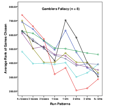
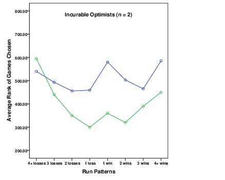
Leopard tested for run effects by conducting a Kruskal Wallis (non-parametric equivalent of ANOVA) analysis of gamble risk for each run length. Runs of losses were coded with a negative run value and runs of gains were coded with a positive run value. A significant run effect was found for 65% of her participants, and each of these participant’s data are summarized in Figure 1. Leopard then grouped participants on the basis of a visual inspection of the graphs displayed in Figure 1. She inferred that eight participants had followed the gambler’s fallacy (Figure 1a) and three participants had shown the hot hand effect (Figure 1b). She also found two participants who provided non-linear risk preferences, and she labeled these participants as incurable optimists (Figure 1c). She believed that these participants increased their risk, because they perceived long runs of any type to signal that a positive outcome is imminent.
Figure 1a: The gambler’s fallacy pattern of risk preferences reported by Leopard (1978) and re-plotted here. Each line represents the mean game ranks chosen by one participant for different run sequences. A larger game rank corresponds to a higher perceived riskiness for a gamble choice.

Figure 1b: The hot hand pattern of risk preferences reported by Leopard (1978) and re-plotted here. Each line represents the mean game ranks chosen by one participant for different run sequences. A larger game rank corresponds to a higher perceived riskiness for a gamble choice.
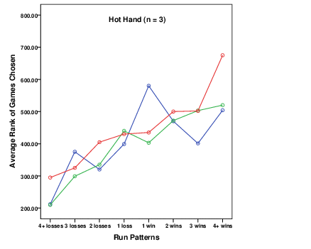
Figure 1c: The “incurable optimists” pattern of risk preferences reported by Leopard (1978) and re-plotted here. Each line represents the mean game ranks chosen by one participant for different run sequences. A larger game rank corresponds to a higher perceived riskiness for a gamble choice.
Leopard’s conclusions raise several questions. Leopard admitted that “Outcome and financial state are inherently confounded to some degree for at least some of the subjects” (p. 525). Many of the participants in Leopard’s study provided significant relationships between risk preference and financial state, including all but three of the participants displayed in Figure 1. In addition, her classification of participants relied solely on visual inspection of the data graphed in Figure 1. However, it is unclear whether the linear and non-linear patterns required for these classifications were actually statistically significant. In addition, consistent trends were not always evident for both types of runs (gains and losses) or across the full range of run lengths. Many of the participants in Figures 1a and 1b showed stronger non-linear trends as run length increased or as run valence changed. Non-linear trends could reflect a change in risk strategy during these times. Finally, the outcomes of each participant’s gambles were random, and therefore the participant’s financial state at the times when runs occurred could have varied dramatically within and between participants. Leopard does not provide any information about how many participants failed to complete the 250 trials or what the financial state of each participant was at the end of each experimental session. It is not out of the question that a participant may have experienced runs only when down from their initial bank, or alternatively, experienced runs only when up from their initial bank. The difficulty with using random event sequences is that there is no control over when runs will occur, what type of run will occur, and how long each run will be.
The goal of the current study is to improve on the Leopard (1978) study by controlling the type of runs, the length of runs, and when these runs occur with respect to the participant’s financial state. A more thorough statistical analysis of the data collected will also provide better justification for the speculated causes of risk preference patterns during runs of gains and losses. I hypothesize that financial status will affect risk preferences, but runs of gains and losses will still influence risk preferences independently of the effects of status. The latter hypothesis is based on the evidence that decision makers are highly predisposed to faulty probabilistic reasoning involving repeated random binary events (Oskarrson, Van Boven, McClelland, & Hastie, 2009). Consequently, linear patterns of risk preferences that follow the gambler’s fallacy (negative slope) and the hot hand (positive slope) are still expected.
However, other participants may show significant non-linear relationships between run variables and risk preference, and there are two possible explanations for these non-linear patterns. Prior research has found that the perceptions of runs may not be linearly related to length. Carlson and Schu (2007) recently reported that an incremental reaction to a sequence of repeated outcomes often peaks at three consecutive outcomes and plateaus after this third event. A second explanation for non-linear effects is that the participant follows different strategies for runs of different lengths and/or valence. For example, the self-perception of being a “lucky winner” after a couple of wins in a row will compete with the growing misperception that this streak must end if it continues to grow. Eventually, the latter perception may win out, and a change in risk preference occurs, leading to a non-linear pattern of risk preferences.
I hypothesize that the use of risk strategies during runs of gains and losses is much more dynamic and transient than suggested by previous research. I expect risk preferences to be influenced in linear and non-linear ways by the valence of runs, the lengths of runs, and the financial status of the individual.
The participants in this study were 60 undergraduate college students (25 males and 35 females) with a mean age of 19.1 years. Participation in this experiment satisfied a course requirement.
A software program written in C+ by the author provided the experimenter-controlled coin toss simulations. Coin tosses were programmed to appear to the participant as random binary events, but this was not the case. Each toss was part of a carefully designed set of toss sequences that served a specific experimental purpose. Some sequences were designed to achieve financial goals and did not contain runs of length greater than two. For example, one goal was to maintain the current financial state of the participant [i.e., P(win) = P(loss)], while other goals involved slowly lowering the participant’s financial state [i.e., P(win) < P(loss)] or slowly raising the participant’s financial state [i.e., P(win) > P(loss)]. Other sequences contained runs of varying length and valence (losses or gains) that ranged from three losses or wins to six losses or wins.
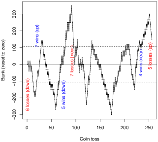
The coin toss simulation program kept a running average (A) for each participant’s bets across the simulated coin tosses. The program then allocated run sequences to satisfy the requirement that runs of varying length and valence (losses and gains) be provided to participants when they were either below their starting bank [bank < ($10.00−3*A)], near their starting bank [($10.00 – 3*A< bank < ($10 + 3*A)], or above their starting bank [bank > ($10.00+3*A)]. For example, if a run of six losses were selected to occur when the participant’s bank was up, the program would manipulate the win/loss ratio for the tosses that preceded this run so that, even after the sixth loss in a row, the participant’s bank would still be greater than $10.00+3*A. Sometimes this meant the participant received a long sequence of coin tosses that slowly manipulated his or her bank, if the financial state required for this run was very different from that required for the previous run. For example, when a run presented at financial state “down” was followed by a run at financial state “up”. On other occasions, the sequence of trials between consecutive runs was much shorter. For example, when a run presented at financial state “down” was followed by a run at financial state “near” the starting bank. The program randomly selected a run each time from the six possible conditions of financial state (start, above, below) and run valence (losses, wins). The run length selected decreased in likelihood as the length of the run increased. For example, a run of length four was three times more likely to be selected than a run of length six. Occasionally a run would result with a length greater than six, because the same run outcome matched one or two tosses that immediately preceded this run. The simulation program continued to cycle through sequences of outcomes in this way until the end of the experiment. Figure 2 provides an illustration of the coin toss outcomes and bets made by one participant. Annotated instances of runs that occurred at each of the six run conditions (financial state and run valence) are also displayed in this figure.
Although the final number of coin tosses varied for each participant, the final bank amount and ratio of wins to losses, was similar for each participant. The participant chose their bets from five choices provided (10c [cents], 20c, 30c, 40c, and 50c) using a computer mouse.
Figure 2: Coin toss outcomes for a participant in the current experiment. Some examples of runs at the various financial state conditions (down, near, or up from starting bank) are annotated. The cut-offs for the financial state conditions are depicted as dashed lines. These cut-offs are not the exact values used for this participant because a running average was calculated for A rather than the final average as depicted here. The bank amount was reset to zero by subtracting $10.00 from the bank variable. The mean bet for this participant was 36 cents. The win/loss ratio was 1.0 and the mean bank was $10.01 for all of the coin tosses.
Participants were tested individually in a small testing room. They sat in front of a computer screen that displayed the outcome of each simulated coin toss. The coin toss task required participants to choose a bet amount from 10 to 50 cents to be gambled on each toss of a computer simulated unbiased coin (Expected Value = 0.0). The starting bank for each participant was $10.00, and the participants were told before starting the simulation that they had a one in five chance of keeping their final bank amount upon completion of the task. On each trial, the participant predicted a coin side for the coin toss, and then selected a bet amount. After a short delay, the computer displayed the result of the simulated coin toss. If the coin side matched the participant’s selection, an auditory series of beeps were emitted and a coin illustration was displayed on the screen. If the coin side did not match the participant’s selection, a low auditory tone was emitted. The participant’s bank was displayed on the screen and adjusted by the amount won or lost. The computer also displayed the results of the last five coin tosses with each win highlighted by a gold circle. The computer simulation manipulated the outcomes of the coin tosses to achieve a balanced range of runs across the three financial state conditions, while still simulating the expected outcomes of a random process. The participant was given a break after runs of varying lengths from all six conditions had been provided (approximately half-way through the experiment). A second phase of coin tosses was then provided to the participant with his or her bank reset back to $10.00 and runs of varying length again allocated randomly across the six run conditions. The experiment could not be completed until a minimum of seven runs for each run condition had been provided over both phases of the experiment, although the time allocated for this experiment usually allowed more runs to be experienced by participants.
After completing the coin toss task, all participants reported that they believed the coin tosses were randomly generated by the computer. One fifth of the participants were randomly selected to receive their final bank amount, and these individuals were paid this amount at the end of the experiment.
Table 1: The relative occurrence of runs of losses and gains after combining data for all participants.
Run type Percentage of occurrence Eight losses 0.1 Seven losses 0.9 Six losses 1.8 Five losses 2.1 Four losses 2.8 Three losses 4.8 Two losses 11.7 One loss 25.6 One win 26.0 Two wins 12.8 Three wins 5.0 Four wins 2.8 Five wins 1.8 Six wins 0.9 Seven wins 0.3 Eight wins 0.1
Figure 3a: Ten participants only provided significant positive linear trends in their risk preferences during runs of gains and losses.
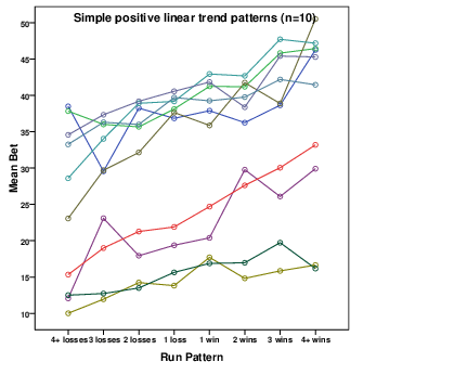
Figure 3b: Twelve participants also displayed significant positive linear trends in their risk preferences, but they also displayed other significant higher order trends as well.
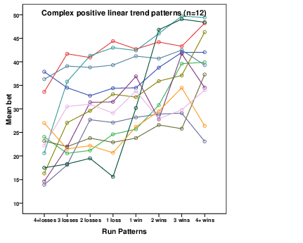
Figure 3c: Four participants only provided significant negative linear trends in their risk preferences during runs of gains and losses.
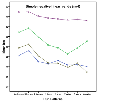
Figure 3d: Three participants also displayed significant negative linear trends in their risk preferences, but they also displayed other significant higher order trends as well.
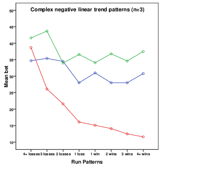
Figure 3e: Seven participants only provided significant quadratic trends in their risk preferences during runs of gains and losses. Six participants revealed negative quadratic trends and one participant a positive quadratic trend.
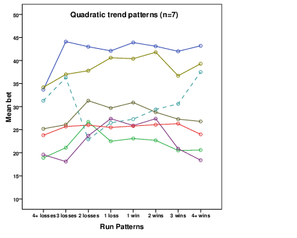
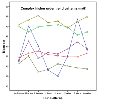
Figure 3f: Six participants provided significant higher order trends (i.e., all significant polynomial degrees greater than two) in their risk preferences during runs of gains and losses.
The mean number of gambles completed by each participant was 252. The mean number of runs with a minimum length of three that participants experienced was 60. The participants’ financial states were recorded as their bank prior to making a bet. The run variable combined length of the run (number of consecutive prior trials of the same outcome) with the valence of the run (gain vs. loss). For example, a run of four prior losses was assigned a value of −4 for this variable, whereas a run of three prior gains was assigned a value of +3 for this variable. Table 1 provides the relative frequencies of trials for runs of specific lengths and valence.
Runs were programmed to occur with similar frequencies for each of the financial state conditions. Consequently, the final bank amount for all participants (M =$10.06; SD = $0.84) did not vary significantly from the participant’s starting bank of $10.00, t(59) = 0.58, p>.05. However, there was still a weak positive correlation between the run variable and the financial status of the participant at the time of the run. Combining the data from all 60 participants revealed a small positive correlation, r(15,431) = 0.13, p<.001; r2 = 0.02.
For this reason, ANCOVA analysis was conducted for each participant, with bet amount as the dependent variable, the run variable tested as a fixed effect, and the participant’s bank amount set as a covariate. Runs that were greater than equal to a length of four were collapsed into one category. This replicated the run categories used by Leopard (1978) and avoids using categories with lower frequencies of occurrence. Polynomial contrasts (first degree to seventh degree) were analyzed to distinguish different patterns of linear and non-linear risk preferences.
One participant was rejected because he failed to vary his bet amounts during the experiment. Significant contrasts were found for 42 (72%) of the remaining 59 participants. Ten participants revealed a simple positive linear trend consistent with the hot hand effect (refer to Figure 3a), however another 12 participants showed more complex positive linear trends with other significant higher degree trends (refer to Figure 3b). These patterns may have been labeled as examples of the hot hand effect by Leopard (1978), but it is quite evident that the risk preferences of these participants are affected by the type of run and the length of the run in ways that are not consistent with following only a simple hot-hand strategy.
Four participants produced a significant linear trend with a negative slope that is consistent with the gambler’s fallacy (refer to Figure 3c). However, another three participants showed more complex negative linear trend patterns that included other significant higher degree trends (refer to Figure 3d). These patterns highlight the difficulty in simply labeling any negative trend as a gambler’s fallacy, because, again, the risk preferences of these participants were affected by the valence of the run and the length of the run.
One participant displayed the positive quadratic trend of risk preferences that Leopard labeled as incurable optimism (refer to Figure 3e). However, the inverse quadratic trend was found for six participants in the current experiment, and this pattern of risk preferences was not reported at all by Leopard (1978) (Figure 3e). Perhaps, Leopard would have classified this latter group as “incurable pessimists”, because they generally decrease their risk as the run length increases (irrespective of run valence). It would seem premature to describe these risk preferences in terms of optimism and pessimism. We can infer only that all of these individuals showed a sensitivity to run length, but not to run valence.
Individual differences in risk preferences during runs of losses and gains are even more idiosyncratic than suggested by previous research, as seven participants showed complex patterns of risk preferences with trends that did not involve any significant linear or quadratic components (Figure 3f). Some participants provide risk preference patterns that appear to reveal complex interaction effects of run length and run valence, while other participants provide simpler symmetrical risk preference patterns that highlight the same run length effects for both types of runs.
The current findings highlight that a larger range of individual differences in risk preferences is possible during runs of gains and losses than has been suggested by previous real-world and laboratory-based research. Risky choices can be influenced by financial status, valence of previous outcomes, and number of consecutive prior outcomes at the time of making this choice. The next step in this statistical analysis is to examine whether there are any overall patterns for these effects on risk preferences during runs of gains and losses.
An exploratory factor analysis was conducted using the predicted effects of run variables and a financial state variable on each participant’s risky choices (bet amounts) in this data analysis. The predicted effects of these variables were determined by conducting a separate multiple regression for each participant using the full range of run lengths as a predictor. Thus I did not restrict the run length to four categories, as in the previous analysis and that of Leopard (1978). The bet amount was the dependent variable in each regression, with the following six variables included as predictor variables: sign (previous outcome was a win or loss), run length (regardless of whether it was a run of losses or gains), quadratic run length (run length squared), signed run length (negative values for runs of losses and positive values for runs of gains), signed quadratic run length (negative values for runs of losses and positive values for runs of gains), and financial status (bank amount with zero defined as the base amount). Quadratic terms were included in these multiple regressions, because many of the participants revealed quadratic trends in the ANCOVA analyses reported previously.
The resulting six unstandardized regression coefficients obtained from each participant’s multiple regression were included as input variables in the exploratory factor analysis. A principle components extraction procedure revealed two factors that produced eigenvalues greater than one. The first factor accounted for 51% and the second factor another 32% of the variance in the regression predictor variables. An oblique rotation was conducted to achieve the final factor loadings, because these factors showed some degree of correlation (r = −.18). The factor loadings are displayed in Table 2, and depict two very distinct sets of risk influences during runs of gains and losses. The first factor was highly influenced by the valence of prior outcomes (sign) with an overall preference for riskier choices after wins than after losses. However, this valence effect varied as a function of the number of prior consecutive outcomes, and changed in slope or direction as the run grew in length or varied in valence. Not only did this factor highlight a complex interaction of run valence and run length on risk preferences during runs of gains and losses, but it also revealed an effect of financial status on risk preferences. Participants who scored high on this factor would risk more when financially down than when financially up. This pattern of risk effects highlights how the win/loss frame of reference for each risky choice can be framed in terms of the outcome result (gain v loss) or the financial consequence of this outcome result.
The second factor loadings reveal a much simpler pattern of effects on risk preferences with a primary focus on the length of the run, regardless of the valence of the run or the financial status of the individual. The opposite sign of the factor loadings for the linear and quadratic trends again suggest a change in risk strategy as the run length increases.
Table 2: Factor loadings for exploratory factor analysis with oblique rotation of multiple regression coefficients for predicting risk preference during runs of gains and losses.
Runs of consecutive gains and losses clearly affect the risky choices of decision makers. Their occurrence can signal to the decision maker that a predictable outcome will occur, even when this predictability is an illusion for random (or near random) events. Decision makers can incorrectly perceive a run of outcomes to be more likely to continue (positive recency; hot hand effect) or to stop (negative recency; gambler’s fallacy), and this misperception gets stronger as the run length increases. Runs of gains and losses also affect the financial state of decision makers, and these financial changes can influence the riskiness of choices made during a run. These dual effects can make distinguishing the reasons for a pattern of risk references that result during a run quite difficult to interpret. For example, increasing the riskiness of choices during a run of wins can be predicted by the hot hand effect or by risking more when financially “up” (gamblers refer to this as playing with the “house” money). Clearly, the same pattern of risk preferences during runs could be motivated by very different thought processes.
The first step in resolving this dilemma was to remove the confounding effect of financial status when examining the effects of run characteristics (length and valence) on risky choices. Previous research has failed to remove this confound, and therefore it is difficult to fully support the strong emphasis on biased reasoning explanations for run effects that have dominated this research area (Ayton & Fischer, 2004; Johnson, Tellis, & MacInnis, 2005; Leopard, 1978; Sundali & Croson, 2006). However, even after controlling for financial state changes during runs, patterns of risk preferences were found in the current study for the majority of participants that are predicted by the hot hand effect or the gambler’s fallacy. This does not rule out the influence of financial state during a run of gains and losses, because this variable was also an additional significant predictor of riskiness for the majority of these participants.
The landmark study by Leopard (1978) suggested there were three patterns of risk preferences during runs of gains and losses (refer to Figure 1) after visually inspecting participants’ risk preferences during runs of various length and valence (gain v loss). However, the current study revealed a much more complex set of risk patterns than just the three singled out by Leopard. These patterns were distinguished by statistical analysis rather than by visual inspection. In addition, these statistical analyses controlled for the confounding change in financial status that occurs during runs. Furthermore, the controlled design of the current study maintained a full range of runs (valence x length) across different financial states (down, near, or up from starting bank).
The current study did find support for Leopard’s previous three groupings with some participants showing only linear risk patterns (Figures 3a and 3c) and one participant showing only a positive quadratic pattern (Figure 3e). The hot hand effect was more evident in the current study than in Leopard’s study, and this could reflect the increased involvement of the participant in the choices involved in the current study. In the current study, the participants chose both the level of risk and coin side on each simulated coin toss. Ayton and Fischer (2004) provide compelling evidence that the presence of the hot hand effect increases in decision tasks with more human involvement in the choice or judgment, than when non-human (e.g., computer) mechanisms solely underlie event outcomes.
Although, there was some support for Leopard’s groupings of risk patterns, many more statistically significant patterns of risk preferences were obtained in the current study (refer to Figures 3b, 3d, 3e, and 3f). The complex nature of risk preferences during runs of gains and losses was further highlighted by an exploratory factor analysis which included the predicted effects of five run variables and financial status on risk preferences as input variables. Predicted effects (i.e., regression weights) were determined by multiple regressions conducted for each participant to predict their risk preferences. The most complex factor explained 51% of the variance in the predicted effects on risk preferences and highlighted the sign of the previous outcome, the run length of previous outcomes (signed for losses and gains), the quadratic run length (signed for losses and gains), and the financial status at the time of the choice. This factor clearly illustrates the complex set of influences on risky choices that can result during runs of gains or losses. Although, a simpler set of effects can also suffice for some individuals. This was evident in the second factor of the exploratory factor analysis that explained an additional 31% of the variance in predicted effects on risky choices. The loadings for this factor only related to the length of the run (regardless of valence), but with opposing linear and quadratic effects for run length (as did Factor 1). These results again suggest a consistent risk strategy was not followed across the full length of the run.
What is not clear however is why one risk strategy or heuristic is preferred for different lengths of runs or for runs of different valence? One possible explanation alluded to by Carlson and Shu (2007), is that runs are identified only after around three consecutive outcomes, and this assumption is consistent with the timing of many changes in risk preferences reported in the current study. However, this explanation does not account for changes in risk preferences as a function of run valence. An additional explanation is needed that attributes risk changes to differences in the motivational influence of thoughts and emotions; both integral to risky choice. For example, the misperception that outcomes of random events are self-correcting may give into the euphoria of winning more and more money as a run continues. Future research could examine these alternative explanations for the dynamic and transient nature of risk preferences during lengthy runs of gains and losses.
The findings of the current experiment highlight the difficulty with inferring the causes underlying risk preferences during runs of gains and losses solely from the risky choices made during such runs. One way to overcome this difficulty is to introduce the qualitative methodology used by Johnson and colleagues in their study. Johnson, Tellis, and Macinnis (2005) asked each participant to provide a reason for a hypothetical investment decision that occurred immediately after a run of gains or losses for this stock. Many of their participants alluded to the gambler’s fallacy or the hot hand when describing their thought processes. But the participants in the Johnson, Tellis, and Macinnis (2007) study only made one decision, whereas the participants in the current study were required to making hundreds of decisions. Some form of sampling procedure would need to be implemented to overcome the larger set of decisions involved in sequential risky choice. The reasons provided by participants could then be coded in terms of reasoning biases, affect-based influences, and financial motivations.
In conclusion, runs of gains and losses are similar to other runs of binary events that result from random (or near random) processes—they are inevitable, they are salient, and they provide an illusion of predictability regarding their continuation. But runs of gains and losses are also different from other runs of binary events that can result from random (or near random) processes—they involve an outcome that not only signals success or failure but also directly affects the decision maker’s assets. It is this added complexity that makes explaining individual differences in risky choice patterns during runs of gains and losses so challenging. The new field of behavioral finance has highlighted the growing interest in predicting investment decisions that result from market trends, yet there is still very little empirical literature (Murstein, 2002). Laboratory simulations like the present one can help to bridge this empirical gap.
Ayton, P., & Fischer, I. (2004). The hot hand fallacy and the gambler’s fallacy: Two faces of subjective randomness? Memory & Cognition, 32, 1369–1378.
Carlson, K. A. & Shu, S. B. (2007). The rule of three: How the third event signals the emergence of a streak. Organizational Behavior and Human Decision Processes, 104, 113–121.
Johnson, J., Tellis, G. J., Macinnis, D. J. (2005). Losers, winners, and biased trades. Journal of Consumer Research, 32, 324–329.
Leopard, A. (1978). Risk preference in consecutive gambling. Journal of Experimental Psychology: Human Perception and Performance, 4, 521–578.
Murstein, B. I. (2002). Getting psyched for Wall Street: A rational approach to an irrational market. Leawood, KS: Cypress Publishing Group.
Oskarsson, A. T., Van Bowen, L., McClelland, G. H., & Hastie, R. (2009). What’s next? Judging sequences of binary events. Psychological Bulletin, 135, 262–285.
Shefrin, H. (2000). Beyond greed and fear: Understanding behavioral finance and the psychology of investing. Boston, MA: Harvard Business School Press.
Sundali, J., & Croson, R. (2006). Biases in casino betting: The hot hand and the gambler’s fallacy. Judgment and Decision Making, 1, 1–12.
This document was translated from LATEX by HEVEA.