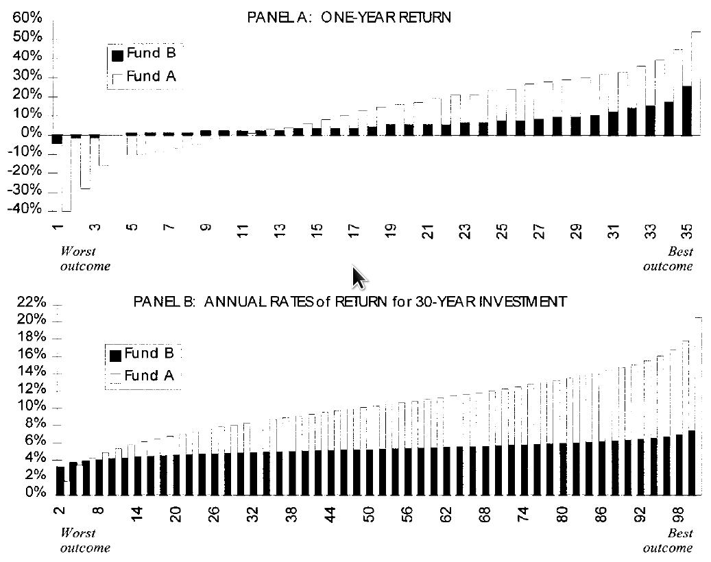
| Figure 1: Graphical return information taken from Benartzi and Thaler (1999). |
Judgment and Decision Making, Vol. 8, No. 5, September 2013, pp. 617-629
Myopic loss aversion: Potential causes of replication failuresAlexander Klos* |
This paper presents two studies on narrow bracketing and myopic loss aversion. The first study shows that the tendency to segregate multiple gambles is eliminated if subjects face a certainty equivalent or a probability equivalent task instead of a binary choice. The second study argues that the behavioral differences previously attributed entirely to myopic loss aversion are partly because long-term return properties are simply easier to grasp if the return information is already provided in the form of long-term returns rather than one-year returns. Both results may be related to recent failures to replicate myopic loss aversion. When the choice situation is structured in such a way that it draws respondents’ attention to the final outcome distribution and/or if severe misestimations of long-term returns based on short-term return information are unlikely, behavioral differences consistent with myopic loss aversion are less likely to be observed.
Keywords: multiple prospects, aggregation, segregation, myopic loss aversion, narrow bracketing.
Redelmeier and Tversky (1992) asked college students if they would like to take a gamble that is independently repeated five times. The one-shot prospect offered a gain of $2,000 and a loss of $500 with equal probability. Sixty-three percent of respondents accepted the repeated gamble when this segregated description was used. Another group of students was offered the following one-shot gamble: a 3% chance to gain $10,000; a 16% chance to gain $7,500; a 31% chance to gain $5,000; a 31% chance to gain $2,500; a 16% chance to gain nothing; and a 3% chance to lose $2,500. Eighty-three percent accepted the gamble when it was presented in this aggregated form.
The gambles are economically identical and differ only in their description. These results suggest that people tend to evaluate one segregated prospect instead of evaluating the aggregated distribution that results from multiple plays. The tendency to segregate multiple prospects can be interpreted as one example of narrow bracketing, a situation where a “decision maker who faces multiple decisions tends to choose an option in each case without full regard to the other decisions and circumstances that she faces” (Rabin and Weizsäcker, 2009, p. 1508; see also Tversky and Kahneman, 1981, and Kahneman and Lovallo, 1993, among others, for further evidence on narrow bracketing).
The idea that multiple gambles are not evaluated based on the aggregated distribution has received considerable attention in economics and finance. The distribution of annual stock returns exhibits a substantial probability of a loss that may make the distribution unattractive for a loss-averse individual. However, an aggregated distribution that can be expected for a long-term investment horizon shows only a small probability of a loss. If loss-averse long-term investors must choose between a stock and a bond portfolio, they are more likely to choose the stock portfolio if aggregated long-term distributions are presented. Benartzi and Thaler (1995) provided field evidence in favor of this combination of narrow bracketing and loss aversion, which they dubbed “myopic loss aversion.”
The concept of myopic loss aversion has been the subject of a number of experimental studies. These studies can be roughly sorted into two groups. The starting point for the first type of experiment was Gneezy and Potters (1997). Subjects were asked to allocate a given amount of money between a risky and a risk-free investment alternative in a multi-period framework. One group received feedback after each period; another group received feedback after three periods. Through less frequent feedback, Gnezzy and Potters (1997) manipulated the degree of narrow bracketing. This study and subsequent experimental studies have found evidence consistent with myopic loss aversion (see Bellemare et al., 2005; Haigh and List, 2005; Fellner and Sutter, 2009, among others).1 I will call this the feedback frequency approach.
A second approach to investigating myopic loss aversion has received less attention. This approach started with Benartzi and Thaler (1999). They asked respondents to make a hypothetical asset allocation decision between a high-risk (stocks) and a low-risk (bonds) fund for a 30-year investment horizon. One group received a graphic with the historic one-year returns of both investment alternatives, sorted separately from the worst one-year return to the best one-year return for each fund. Another group received a graphical representation of simulation results. To generate them, the authors drew 30 one-year returns from the historical one-year returns with replacement. Afterwards, they calculated the annualized return for the hypothetical 30-year time period. Repeating this procedure 10,000 times yielded the distribution for the second presentation format. Narrow bracketing should be reduced under the latter presentation format. Additionally, subjects should realize that stocks are unlikely to generate any losses over a 30-year investment horizon. The original graphics for both presentation formats used by Benartzi and Thaler (1999) are reproduced in Figure 1. Consistent with myopic loss aversion, respondents invested significantly more in stocks (Funds A in Figure 1) when the annualized 30-year returns were presented. I will call this the distribution approach.
Figure 1: Graphical return information taken from Benartzi and Thaler (1999).
The experimental evidence reported in early studies was typically consistent with myopic loss aversion. However, recent studies have found evidence that seems to be at odds with the theory. Moher and Koehler (2010) were able to replicate the results of Gneezy and Potters (1997) by using their original design, but they failed to observe behavior consistent with myopic loss aversion if they played similar gambles instead of the same gambles repeatedly. They furthermore found no evidence of myopic loss aversion when respondents had to choose between two gambles instead of making an asset allocation decision. Glätzle-Rützler et al. (2013) found no evidence of myopic loss aversion in a sample of 755 adolescents (aged 11 to 18 years) using the original Gneezy and Potter (1997) design.
With respect to the distribution approach, Beshears et al. (2012) found no effect of aggregating return information on behavior. This result is surprising because they used essentially the same graphical presentation format as Benartzi and Thaler (1999). Participants from a non-student subject pool were asked to allocate $325 among four real-world investment funds with a one-year investment horizon. These participants, older than 25 years and with an annual income of at least $35,000, received the value of the portfolio after one year.
There are many potential explanations for the conflicting results. In this paper, I investigate two conditions under which myopic loss aversion is mitigated. I start by arguing that seemingly minor differences in decision tasks can cause a significant difference in results. In theory, every aspect of a decision task that mitigates narrow bracketing should also reduce the influence of myopic loss aversion. Study I in this paper presents evidence in favor of this hypothesis by using a seemingly minor modification of the design of Redelmeier and Tversky (1992).
The second study in this paper addresses the distribution approach. Differences in behavior between the groups who had seen one-year returns and simulated 30-year returns can be caused either by myopic loss aversion or by severely misestimating long-run returns based on the one-year returns in the former group. Previous research has shown that people have difficulty predicting the distributional features of repeated gambles based on information about the one-shot distribution (see Klos et al., 2005; Stutzer and Grant, 2013) and that there is a general tendency to misestimate long-term results if asset values grow exponentially (Stango and Zinman, 2009).
Furthermore, the literature suggests that people are more willing to take risks if they have a solid understanding of the underlying decision problem. Heath and Tversky’s (1991) competence hypothesis states that “people prefer to bet in a context where they consider themselves knowledgeable or competent than in a context where they feel ignorant or uninformed” (p. 7). Consistent with this idea, studies of financial decision making have shown that individuals with a low degree of financial literacy show more risk-averse behavior (see Wang, 2009; van Rooij et al., 2011).
There are therefore two channels through which severe misestimations can induce a lower willingness to take risks in the segregated condition of the distribution approach. First, if the perceived return difference between stock and bond returns is smaller in the segregated condition, people may choose a smaller exposure to equities because of the lower perceived return prospects of stocks. Second, consistent with the competence hypothesis, respondents will choose less risky allocations in the segregated condition because they were not able to build reasonable estimates of the basic long-term return properties of the offered funds, thereby exhibiting a reduced perceived competence in comparison to subjects in the aggregated condition. Note that the second channel could also lead to a decreased willingness to take risks if participants are overestimating the long-term prospects of stocks relative to those of bonds.
Study II in this paper presents evidence that there are more respondents with severe misestimations in the segregated condition and that people exhibiting such misestimations choose less risky allocations. These two effects together cause a difference in the observed risk taking in the aggregated and segregated condition, which is not caused by a framing mechanism as hypothesized by myopic loss aversion.
Procedure: I consider a slight modification of the original design of Redelmeier and Tversky (1992) to test the hypothesis that the decision task itself influences people’s tendency to segregate. The experimental variation that is expected to decrease the tendency to bracket narrowly is to ask for a certainty equivalent or for a probability equivalent instead of a binary choice of whether or not respondents would like to take the gamble. Compared with a simple binary choice situation, it is likely that the necessity to write down a number in the certainty and the probability equivalent tasks forces respondents to think more thoroughly about the decision problem and thereby about the aggregated outcome distribution.
I replicated Redelmeier and Tversky’s (1992) study (labeled “Choice,” columns 2 and 3 in Table 1) and conducted slightly extended versions that ask for a certainty equivalent (labeled “Certainty Equivalent,” columns 4 and 5 in Table 1) or a probability equivalent (labeled “Probability Equivalent,” columns 6 and 7 in Table 1). In the certainty equivalent task, participants were asked to state the amount of money CE that makes a respondent indifferent between playing the prospect and receiving CE. The concept of the certainty equivalent was discussed in class as part of the lecture before the questionnaire study. In the probability equivalent task, respondents compared the aggregated or the segregated prospect of Redelmeier and Tversky (1992) to another lottery L. This lottery L offered a gain of 10,000 euros with a probability p and a loss of 2,500 euros with a probability 1-p. Participants were asked to state the probability p that makes her/him indifferent between playing the prospect and playing lottery L.
Subjects: In line with Redelmeier and Tversky (1992), I deliberately conducted a between-subject questionnaire study without monetary incentives, using undergraduates as participants. Deviations from rational behavior may be more likely in such an environment (see, e.g., Ortmann & Hertwig, 2001). If this is generally true, experimental manipulations are more likely to change behavior. As a consequence, differences in the certainty and probability equivalent tasks are more likely to be observed.
In total, 404 students participated. Students in the binary and certainty equivalent tasks were participants of an introductory Bachelor’s course on decision analysis at the University of Kiel. Respondents were either Bachelor’s students on a decision analysis course or Master’s students on a behavioral finance course in the probability equivalent task. The questionnaire was carried out in the teaching language of the course, which was German on the Bachelor’s and English on the Master’s courses. Roughly 50% of participants in the behavioral finance class were foreign students whose first language was not German. The observations from Master’s and Bachelor’s students exhibited the same pattern.
Result 1.1: There is a difference between the acceptance rates in the binary choice task (replication of Redelmeier and Tversky, 1992).
In the choice task, 75.4% (N=69) of respondents would take the gamble under the segregated presentation format, whereas 92.4% (N=66) accepted the aggregated gamble. The null hypothesis that both samples come from the same population can be rejected (p=0.0075; Mann-Whitney U-test). This result is consistent with Redelmeier and Tversky (1992), although the respondents in my sample behaved less risk-averse on average (see Table 1).
Table 1: Results of Study I.
Choice Certainty Eq. Probability Eq. 0.0075 0.8486 0.1776 Note: N denotes the number of respondents in each condition. p stands for the p-value belonging to a non-parametric Mann-Whitney U-test. The percentage number in the choice condition gives the percentage of respondents that accepted the prospect. The percentage number in the probability equivalent condition is the average stated probability that makes a respondent indifferent between the offered gambles.
Result 1.2: There is no difference between the certainty (probability) equivalents in the certainty (probability) equivalent task.
The picture changes if respondents are asked to state their certainty equivalent. There is only a tiny and insignificant difference between an aggregated (2,954.25 euros; N=60) and a segregated (2,987.65 euros; N=81) description. The implicit acceptance rates, i.e., the percentage of respondents that stated a certainty equivalent greater than zero, are 91.7% (aggregated) and 93.8% (segregated). These numbers are very close to the 92.4% of the aggregated representation in the choice task. The upper panel of Figure 2 shows the empirical cumulative distribution functions of the certainty equivalents for the aggregated and segregated descriptions. Both distributions are similar.
Figure 2: Results of Study I: Cumulative distribution functions for the certainty and probability equivalents. 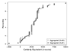
Note: Shown are the empirical cumulative distribution functions, defined as the proportion of certainty (probability) equivalent values less than or equal to a given certainty (probability) equivalent.
As the responses of the certainty equivalent task can be interpreted as implicit acceptance rates, it is possible to explicitly test for an interaction effect. I estimate the following logistic regression (N=276):
|
where Acceptance is a dummy variable that is equal to 1 if the prospect is accepted and 0 otherwise, x1 is a dummy variable that is equal to 1 if the prospect was presented in the segregated description and 0 otherwise, x2 is a dummy variable that is equal to 1 if the observation comes from the choice treatment and 0 otherwise, and x3 is the interaction between both dummy variables. Reported are the coefficients for the latent variable. Standard errors are in brackets. There is a significant interaction effect (p=0.045). The coefficient of the framing dummy (x1) is positive, but not significantly different from zero (p=0.622).
Table 1 also shows the results of the probability equivalent task. Myopic loss aversion predicts that the prospect is more attractive under an aggregated description, implying that the probability that makes a respondent indifferent is larger in the aggregated than in the segregated treatment. The average probability equivalent is 60.0% (N=61) under the aggregated and 53.6% (N=67) under the segregated description. However, the difference is not statistically significant (p=0.1776; Mann-Whitney U-test). The lower panel of Figure 2 shows the empirical cumulative distribution function for the probability equivalent questions. The distributions are again similar and mirror the insignificantly higher probability equivalents in the aggregated treatment. More respondents chose 50% in the segregated treatment, suggesting that more people matched expected values under the segregated description. A formal interaction analysis cannot be conducted, as there is no way to deduce an implied acceptance rate from the probability equivalents.
Procedure: I used the graphics used by Benartzi and Thaler (1999), as shown in Figure 1.2 The group that had seen only one-year returns (simulated 30-year returns) is called the segregated (aggregated) group or is acting under the segregated (aggregated) condition. Respondents were told that they should assume that the past is representative of the future.
The key difference to Benartzi and Thaler’s (1999) study is that some respondents had to answer two short estimation questions before they stated their asset allocations for the 30-year horizon. Respondents were asked to estimate the amount of money to which one euro invested today would grow in 30 years. One estimate should be stated for each fund. Respondents were allowed to use a calculator and many of them did.
Subjects: I again used an undergraduate subject pool without monetary incentives. Benartzi and Thaler (1999) used (non-faculty) staff employees at the University of Southern California and did not use incentive-compatible payment. It seems likely that the math and statistics skills that are necessary for the estimation tasks are more developed in the student population, although this is an ex-post, untestable hypothesis.
A total of 152 students answered the allocation question without any estimation tasks. Altogether, 78 (74) of them were exposed to the segregated (aggregated) description. 198 were additionally asked to answer the two estimation questions. 95 (103) of them responded to the segregated (aggregated) description. All students came from introductory Bachelor’s courses on finance and decision analysis at the University of Kiel. One respondent who stated that a euro invested in bonds will result in a negative amount of money after 30 years is excluded from the data analysis.
Result 2.1: Equity exposure is higher in the aggregated than in the segregated condition (replication of Benartzi and Thaler, 1999) if the pooled data is used.
Students who had seen the aggregated 30-year information allocated 64.8% (N=177) to stocks, while those confronted with the segregated one-year information allocated 57.7% (N=173) to stocks (p=0.0092, Mann-Whitney U-test). This result is qualitatively consistent with previous research, although the effect size is considerably smaller than in Benartzi and Thaler (1999), where USC staff employees (nonfaculty) allocated on average 82% in the aggregated and 42% in the segregated condition to the risky asset.
Result 2.2: There is no significant difference in the subsample of respondents who were asked to additionally respond to the estimation questions. However, this observation does not translate into a significant interaction effect between asking estimation questions and the information format.
The difference between average allocations in the subsample of respondents asked the estimation questions is somewhat smaller (segregated: 63.0%, N=95; aggregated: 68.2%, N=103). The null hypothesis of equal distributions cannot be rejected using a Mann-Whitney U-test (p=0.1693). To explicitly test for an interaction effect, I estimate the following Tobit model, where the dependent variable (allocation to risky assets) is censored from above (100) and below (0) (N=350):
|
where x1 is a dummy variable that is equal to 1 if the return information was presented in the segregated description and 0 otherwise, x2 is a dummy variable that is equal to 1 if the observation comes from the condition with the estimation questions and 0 otherwise, and x3 is the interaction between both dummy variables. Standard errors are in brackets. There is no significant interaction effect (p=0.524).
Result 2.3: The estimated return difference in the aggregated condition is larger than the estimated return difference in the segregated condition.
A total of 185 students answered both estimation questions in addition to the allocation question, namely 93.4% (=185/198) of the students asked to answer the estimation questions. The elicited values are the value of one euro invested over 30 years in either stocks or bonds. I convert these numbers into implied annualized returns according to following formula. If v30 is the value of a euro after 30 years, the implied annualized return is equal to r30=(v30)1/30−1. Figure 3 shows the distribution of implied returns for stocks and bonds as well as the difference in implied returns.
Figure 3: Results of Study II: Cumulative distribution functions for implied annualized returns. 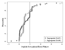
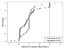
Note: Shown are the empirical cumulative distribution functions, defined as the proportion of returns less than or equal to a given return.
The average implied return for bonds (stocks) is 6.7% (9.3%) in the segregated and 6.6% (10.1%) in the aggregated condition. There is a considerable amount of unreasonable high and low estimates in both conditions. In the aggregated condition, many respondents estimate the implied stock return to be roughly 10% and the implied bond return to be roughly 4%-5%. The average implied return difference is 2.6% (3.4%) in the segregated (aggregated) condition. The difference in medians is considerably larger (segregated: 0.6%; aggregated: 4.0%). The null hypothesis of equal distributions can be rejected (p=0.0205; Mann-Whitney U-test).
Result 2.4: A larger proportion of people with severe misestimations are observed under the segregated condition than under the aggregated condition.
To understand how important bounded rationality in this context is, I classify a reasonable answer to the estimation questions based on three criteria. First, respondents should understand that stocks outperform bonds. Equivalently, they should understand that the implied return difference is larger than zero. Second, respondents should realize that the implied stock return is smaller than 30%. Third, respondents should realize that the implied bond return is smaller than 10%. Higher bounds are chosen based on the observation that even a willing eye cannot determine more than 10 out of the 35 bars in the graphical description in the segregated condition that lie above or are equal to 30% for stocks (10% for bonds). Furthermore, there is a substantial number of negative returns for both asset classes. Estimates above 30% for stocks or above 10% for bonds can therefore arguably be classified as unreasonable in the segregated condition. In the aggregated condition, they are obviously unreasonable because the highest long-term return is slightly above 20% for stocks and roughly 8% for bonds.
If the answers from one person fulfill all three criteria, this respondent is classified as a person with a reasonable understanding of the basic return properties. All boundaries are shown as solid dark lines in the cumulative distribution in Figure 3.
Altogether, 28.8% in the segregated condition and 20.4% in the aggregated condition did not realize that stocks outperform bonds. Further, 33.3% in the segregated condition and 21.4% in the aggregated condition believed that the implied stock return is larger than or equal to 30% and/or that the implied bond return is larger than or equal to 10%.
Combining both criteria yields a proxy for a person with a reasonable understanding of the return properties: 70.4% (N=98) gave reasonable estimates in the aggregated condition but only 49.4% (N=87) did so in the segregated condition (p=0.0037; Mann-Whitney U-test).
Result 2.5: Respondents with reasonable return estimates show less risk-averse behavior than respondents with unreasonable return estimates.
Figure 4: Results of Study II: Average allocations. Note: N in the aggregate condition with an unreasonable estimate: 29; N in the segregated condition with an unreasonable estimate: 44; N in the aggregate condition with a reasonable estimate: 69; N in the segregated condition with a reasonable estimate: 43.
Figure 4 shows the average exposure to stocks for those persons who have a reasonable understanding of the return properties and those who do not. It is obvious that whether or not people are able to give a reasonable return estimate is important for observed allocations. Respondents with a reasonable estimate allocated roughly 75% to stocks, while respondents with an unreasonable understanding of the return properties chose an equity exposure of less than 55%. A Mann-Whitney U-test rejects the null hypothesis of equal distributions in both treatments at the 1% level (p<0.0001 in the segregated condition and p=0.0018 in the aggregated condition).
Result 2.6: The smaller proportion of reasonable estimates in the segregated condition partly accounts for the myopic loss aversion effect.
Result 2.4 (more misestimations in the segregated condition) and Result 2.5 (much lower exposure to equities if unreasonable estimates are observed) suggest Result 2.6 if they are taken together. To investigate this claim further, I perform a standard indirect effect analysis.3 Figure 5 shows the result. Although the total effect is not significant in this subsample (N=185; τ=-5.95; p=0.180), there is a significant indirect effect (see, e.g., Hayes, 2009, for a discussion on how this can easily happen). The point estimate for the indirect effect is -4.95. The 95% confidence interval determined with a percentile bootstrap approach (5,000 repetitions) is [-9.25;-1.49], which indicates that the indirect effect is significantly different from zero.4
Figure 5: Results - Study II: Indirect effect analysis (N=185) 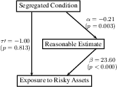
Note: α comes from a linear regression of the reasonable estimate dummy on the treatment dummy. β and τ’ (direct effect) come from a linear regression of the chosen allocation on the reasonable estimate dummy and the treatment dummy.
Remarks on the definition of a reasonable estimate and robustness checks: Three criteria must be simultaneously met in order to classify an implied return difference to be a reasonable estimate. The first criterion (respondents should recognize that stocks outperform bonds) seems to be uncontroversial. However, the thresholds chosen for unreasonable high return estimates are more debatable.
A natural question is how the results would be affected for an alternative upper threshold. I therefore repeat the analysis for Study II with several alternative thresholds. The alternative thresholds for the implied stock (bond) return are 20%, 25%, and 35% (8%, 9%, 11%, and 12%). The results are reported in Appendix A. They are qualitatively unaffected.
One may further argue that the estimation questions are easier in the aggregated than in the segregated condition and that one should therefore consider two alternative thresholds. Although it is almost certainly true that the estimation questions are easier in the aggregated condition, I believe that the comparisons presented so far are more meaningful. It is exactly this feature that motivated Study II, and the primary goal was to assess if this issue is important for the overall myopic loss aversion effect. However, I report additional results in Appendix B for the sake of completeness. For these additional analyses, the thresholds for the segregated condition are at the original levels (30% for stocks and 10% for bonds), while the thresholds for the aggregated condition are 14%, 15%, and 16% for stocks and 5%, 6%, and 7% for bonds. The results are qualitatively similar as long as an implied bond return of 5% is not classified as unreasonable. In light of Figure 1, I do not believe that 5% is an unreasonable estimate in the aggregated condition.
The results of Study I provide evidence for the hypothesis that aspects of the decision task itself influence the tendency to segregate. If the task shifts decision makers’ attention towards the final outcome distribution, the degree of narrow bracketing is reduced, and thereby the importance of myopic loss aversion is mitigated. Asking for a certainty equivalent instead of binary choice is enough to eliminate the framing effect in Redelmeier and Tversky (1992). There is no significant framing effect if a probability equivalent task is used.
There are alternative explanations for the differences in the certainty/probability equivalent and the binary choice task. In general, any satisfying alternative explanation should explain why the observed behavior is only consistent with myopic loss aversion in the binary choice task, but not in the certainty or the probability equivalent task. I will briefly discuss two alternative explanations.
As I use different response modes in Study I, it might be that some form of compatibility effect affects the results. Tversky et al. (1990) and Slovic et al. (1990) offered the compatibility hypothesis, which states that “the weight of a stimulus attribute is enhanced by its compatibility with the response” (Slovic et al., 1990, p. 5), as an explanation of preference reversals. Payoffs may receive greater weight relative to probabilities in the certainty equivalent task compared with binary choices. However, the fact that no significant effect of myopic loss aversion is observed for both certainty and probability equivalents makes it unlikely that some compatibility effect is causing the results.
A potential second explanation starts with the observation that respondents in the certainty equivalent task are asked for a certain amount of money that makes them indifferent to the stated prospect. This question may be interpreted as a hint that the desired number should be positive and an experimenter demand effect could potentially result. Such a demand effect should increase the implicit acceptance rate in both treatments. However, the acceptance rate increases only using the segregated description. Furthermore, such a demand effect could not explain the results in the probability equivalent task.
Based on the results of Study I, one would expect that drawing subjects’ attention towards the final outcome distribution is a potential choice architecture tool (see, e.g., Johnson et al., 2012) for debiasing respondents in the segregated condition in general. However, in the more complicated choice situation that subjects faced in Study II, the data are inconsistent with this conjecture. There is no significant interaction effect between asking estimation questions and presentation format on allocations in an experiment that uses different representations of long-term returns.
Study II further extends the literature that investigates the predictions of myopic loss aversion in the distribution approach. One potential problem with previous research is that it confounds two effects: a framing effect consistent with myopic loss aversion and an effect caused by severe misestimating. Study II shows that respondents who have seen only one-year returns are much more likely to misestimate the basic return properties. These people also choose a less risky asset allocation, presumably because they are aware of their difficulty estimating the long-term return properties and because the underestimation of the implied return difference is more common than is an overestimation. The results of Study II thus suggest that this misestimation can explain a significant part of the differences observed in previous research.
These results have implications for the ongoing discussion about the merits of laboratory studies of “real-world” behavior. One obvious difference between Beshears et al. (2012) and Benartzi and Thaler (1999) is the field context. It is possible that the sizes of the stakes, the non-student subject pool, and/or the one-year duration are responsible for the differences in the presented results. It would be an alarming result for laboratory research in general if the field context were indeed the causal driver. For example, Cox (2011) discussed a former version of the paper by Beshears et al. (2012) in a report for Morgan Stanley and stated that "this closer-to-the-field evidence appears to suggest that practitioners and regulators do not have quite the ability to influence members through information presentation" (p. 17). There is already an active discussion about lab/field generalizability in economics (see Levitt and List, 2007, 2008; Camerer, 2011).
Based on the results presented in this paper, I offer an alternative interpretation that is not based on lab/field differences. Beshears et al. (2012) presented aggregated returns for a five-year period instead of a 30-year period. Severe misestimations are less likely over the much shorter five-year period. Furthermore, the respondents in the sample of Beshears et al. (2012) show a higher degree of financial literacy compared with a representative sample of the American population (see Lusardi and Mitchell, 2011, and Table 4 in Beshears et al., 2012), again making severe misestimations less likely.
Although somewhat speculative, it is also possible that the five-year investment horizon reduces people’s tendency to segregate because it is easier to make reasonable return estimations over five years than it is over 30 years. Generally, further research using the distribution approach should address which features of a long-term investment decision actually influence people’s tendency to segregate. A satisfactory answer would allow a better assessment if risk taking can indeed be influenced by aggregating return information.
From a methodology point of view, it is tempting to conclude that classic experimental research methods are not useful for the question at hand if we see differences between the field and the lab. I would like to stress that the alternative interpretations of the results of Beshears et al. (2012) offered here are based on questionnaire studies with undergraduates, a classic experimental method especially popular in psychology. Many differences exist between the lab and field. Classic experimental methods give us the possibility to investigate a single potential driver of differences in a controlled environment. In this sense, I believe that lab/field differences actually call for more experimental research in the field and in the lab.
Taking the results of both studies together, this paper suggests that myopic loss aversion is less likely to be important if the decision task leads decision makers’ attention towards the final outcome distribution and if decision makers are financially literate and therefore unlikely to be prone to severe return misestimations.
Finally, I would like to stress that the results do not imply that myopic loss aversion is not real; nor do the results of Study II imply that the manipulations in the distribution approach are never causing a framing effect. Such differences may well exist, especially among financially illiterate people.
Benartzi, S., & Thaler, R. H. (1995). Myopic loss-aversion and the equity premium puzzle. Quarterly Journal of Economics, 110, 73–92.
Benartzi, S., & Thaler, R. H. (1999). Risk aversion or myopia? Choices in repeated gambles and retirement investments. Management Science, 45, 364–381.
Bellemare, C., Krause, M., Kröger, S., & Zhang, C. (2005). Myopic loss aversion: Information feedback vs. investment flexibility. Economics Letters, 87, 291–439.
Beshears, J., Choi, J. J., Laibson, D., & Madrian, B. C. (2012). Does aggregated returns disclosure increase portfolio risk-taking? Yale University, Retrieved July 19, 2013, from http://faculty.som.yale.edu/jameschoi/aggregation.pdf.
Camerer, C. (2011). The promise and success of lab-field generalizability in experimental economics: A critical reply to Levitt and List. CalTech, Retrieved July 19, 2013, from http://papers.ssrn.com/sol3/papers.cfm?abstract_id=1977749.
Cox, P. (2011). The provision of information to members of defined contribution schemes: A review of existing research. University of Birmingham, Report prepared for JP Morgan. Retrieved July 19, 2013, from http://www.birmingham.ac.uk/Documents/college-social-sciences/social-policy/CHASM/provision-information-members-defined-contribution-schemes.pdf.
Fellner, G. & Sutter, M. (2009). Causes, consequences and cures of myopic loss aversion - An experimental examination. Economic Journal, 119, 900–916.
Fritz, M. S., Taylor, A. B., & MacKinnon, D. P. (2012). Explanation of two anomalous results in statistical mediation analysis. Multivariate Behavioral Research, 47, 61–87.
Glätzle-Rützler, D., Sutter, M., & Zeileis, A. (2013). No myopic loss aversion in adolescents? An experimental note, University of Innsbruck, Retrieved July 19, 2013, from http://eeecon.uibk.ac.at/wopec2/repec/inn/wpaper/2013--07.pdf.
Gneezy, U., & Potters, J. (1997). An experiment on risk taking and evaluation periods. Quarterly Journal of Economics, 112, 631–646.
Haigh, M. S., & List, J. A. (2005). Do professional traders exhibit myopic loss aversion? An experimental analysis. Journal of Finance, 60, 523–534.
Hayes, A. F. (2009). Beyond Baron and Kenny: Statistical mediation analysis in the new millennium. Communication Monographs, 76, 408–420.
Hayes, A. F., & Scharkow, M. (2013). The relative trustworthiness of inferential tests of the indirect effect in statistical mediation analysis: Does method really matter? Psychological Science, forthcoming.
Heath, C., & Tversky, A. (1991). Preference and belief: Ambiguity and competence in choice under uncertainty. Journal of Risk and Uncertainty, 4, 5–28.
Johnson, E. J., Shu, S., Dellaert, B. G. C., Fox, C. R., Goldstein, D.G., Hauble, G., Larrick, R. P., Payne, J., Peters, E., Schkade, D., Wansink, B., & Weber, E.U. (2012). Beyond nudges: Tools of choice architecture. Marketing Letters, 23, 487–504.
Kahneman, D., & Lovallo, D. (1993). Timid choices and bold forecasts: A cognitive perspective on risk taking. Management Science, 39, 17–31.
Klos, A., Weber, E. U., & Weber, M. (2005). Investment decisions and time horizon: Risk perception and risk behavior in repeated gambles. Management Science, 51, 1777–1790.
Langer, T., & Weber, M. (2001). Prospect-theory, mental accounting, and differences in aggregated and segregated evaluation of lottery portfolios. Management Science, 47, 716–733.
Langer, T., & Weber, M. (2005). Myopic prospect theory vs. myopic loss aversion - How general is the phenomenon? Journal of Economic Behavior and Organization, 56, 25–38.
Levitt, S., & List, J. A. (2007). What do laboratory experiments measuring social preferences reveal about the real world? Journal of Economic Perspectives, 21, 153–174.
Levitt, S., & List, J. A. (2008). Homo economicus evolves. Science, 319, 909–910.
Lusardi, A., & Mitchell, O. S. (2011). Financial literacy and retirement planning in the United States. Journal of Pension Economics and Finance, 10, 509–525.
Ortmann, A., & Hertwig, R. (2001). Experimental practices in economics: A challenge for psychologists? Behavioral and Brain Sciences, 24, 383–403.
Moher, E., & Koehler, D. J. (2010). Bracketing effects on risk tolerance: Generalizability and underlying mechanisms. Judgment and Decision Making, 5, 339–346.
Tversky, A., & Kahneman, D. (1981). The framing of decisions and the psychology of choice. Science, 211, 453–458.
Rabin, M., & Weizäcker, G. (2009). Narrow bracketing and dominated choices. American Economic Review, 99, 1508–1543.
Redelmeier, D., & Tversky, A. (1992). On the framing of multiple prospects. Psychological Science, 3, 191–193.
Slovic, P., Griffin, D., & Tversky, A. (1990). Compatibility effects in judgment and choice. In R. M. Hogarth (Ed.), Insights in decision making, pp. 5–27. Chicago, IL: University of Chicago Press.
Stango, V., & Zinman, J. (2009). Exponential growth bias and household finance. Journal of Finance, 64, 2807–2849.
Sobel, M. E. (1982). Asymptotic confidence intervals for indirect effects in structural equation models. In S. Leinhardt (Ed.), Sociological Methodology, pp. 290–312. Washington DC: American Sociological Association.
Stutzer, M., & Grant, S. J. (2013). Misperceptions of long-term investment performance: Insights from an experiment. Journal of Behavioral Finance and Economics, forthcoming.
Tversky, A., Slovic, P., & Kahneman, D. (1990). The causes of preference reversal. American Economic Review, 80, 204–217.
van Rooij, M., Lusardi, A., & Alessiee, R. (2011). Financial literacy and stock market participation. Journal of Financial Economics, 101, 449–472.
Wang, A. (2009). Interplay of investors’ financial knowledge and risk taking. Journal of Behavioral Finance, 10, 204–213.
This appendix reports results of robustness checks where the upper thresholds for unreasonable stock and bond returns are varied. As in the main text, one set of thresholds is applied to both conditions.
| Threshold | Percentage of unreasonable | Percentage of | Average allocations | |||||||
| stock/ | high estimates | reasonable estimates | p-value | p-value | unreasonable estimates | reasonable estimates | ||||
| bond return | Agg. | Seg. | Agg. | Seg. | Mann-Whitney-U | t-test | Agg. | Seg. | Agg. | Seg. |
| 20%/8% | 0.306 | 0.437 | 0.643 | 0.437 | 0.005 | 0.002 | 53.714 | 53.884 | 77.067 | 74.25 |
| 20%/9% | 0.306 | 0.402 | 0.643 | 0.46 | 0.013 | 0.006 | 53.714 | 52.198 | 77.067 | 75.213 |
| 20%/10% | 0.245 | 0.356 | 0.673 | 0.471 | 0.006 | 0.003 | 51.156 | 51.159 | 77.246 | 75.817 |
| 20%/11% | 0.224 | 0.322 | 0.673 | 0.494 | 0.014 | 0.007 | 51.156 | 51.212 | 77.246 | 74.616 |
| 20%/12% | 0.214 | 0.31 | 0.684 | 0.494 | 0.009 | 0.004 | 51.194 | 51.212 | 76.84 | 74.616 |
| 25%/8% | 0.286 | 0.425 | 0.663 | 0.448 | 0.003 | 0.002 | 55.455 | 53.34 | 75.465 | 74.397 |
| 25%/9% | 0.286 | 0.391 | 0.663 | 0.471 | 0.009 | 0.004 | 55.455 | 51.594 | 75.465 | 75.329 |
| 25%/10% | 0.214 | 0.345 | 0.704 | 0.483 | 0.002 | 0.001 | 54.379 | 50.518 | 74.757 | 75.917 |
| 25%/11% | 0.194 | 0.31 | 0.704 | 0.506 | 0.006 | 0.003 | 54.379 | 50.542 | 74.757 | 74.739 |
| 25%/12% | 0.184 | 0.299 | 0.714 | 0.506 | 0.004 | 0.002 | 54.536 | 50.542 | 74.404 | 74.739 |
| 30%/8% | 0.286 | 0.425 | 0.663 | 0.448 | 0.003 | 0.002 | 55.455 | 53.34 | 75.465 | 74.397 |
| 30%/9% | 0.286 | 0.391 | 0.663 | 0.471 | 0.009 | 0.004 | 55.455 | 51.594 | 75.465 | 75.329 |
| 30%/10% | 0.214 | 0.333 | 0.704 | 0.494 | 0.004 | 0.002 | 54.379 | 49.621 | 74.757 | 76.244 |
| 30%/11% | 0.194 | 0.264 | 0.704 | 0.552 | 0.032 | 0.016 | 54.379 | 47.777 | 74.757 | 74.969 |
| 30%/12% | 0.184 | 0.253 | 0.714 | 0.552 | 0.022 | 0.011 | 54.536 | 47.777 | 74.404 | 74.969 |
| 35%/8% | 0.276 | 0.425 | 0.673 | 0.448 | 0.002 | 0.001 | 55.625 | 53.34 | 75.08 | 74.397 |
| 35%/9% | 0.265 | 0.391 | 0.684 | 0.471 | 0.004 | 0.002 | 55.161 | 51.594 | 75.004 | 75.329 |
| 35%/10% | 0.194 | 0.322 | 0.724 | 0.506 | 0.002 | 0.001 | 53.963 | 49.845 | 74.342 | 75.42 |
| 35%/11% | 0.173 | 0.23 | 0.724 | 0.586 | 0.048 | 0.024 | 53.963 | 47.87 | 74.342 | 73.304 |
| 35%/12% | 0.163 | 0.218 | 0.735 | 0.586 | 0.033 | 0.016 | 54.115 | 47.87 | 74.003 | 73.304 |
Note: Each row shows the results of one robustness check. The first column lists the alternative thresholds for an absurd high stock and bond return estimate that is used in the robustness check. Columns 2 to 5 show the resulting percentages of unreasonable high return estimates and the resulting percentages of reasonable estimates (excluding also those who did not understand that stocks outperform bonds). The p-value of a Mann-Whitney-U test with the null hypothesis that the distribution of reasonable estimates is equal for both conditions is shown in Column 6. Column 7 shows the p-value of a one-sided t-test with the null hypothesis that the percentage of reasonable estimates is higher in the segregated condition. The remaining columns contain the average allocations of subjects with reasonable and unreasonable estimates under both conditions.
| Indirect effect analysis | ||||||||||
| Threshold | Bootstrapped 95%- | |||||||||
| stock/ | confidence interval (percentile) | |||||||||
| bond return | α | β | τ | τ′ | αβ | Std.Err(αβ) | z-value | p-value | Lower bound | Upper bound |
| 20%/8% | −0.206 | 21.897 | −5.948 | −1.435 | −4.512 | 1.806 | −2.499 | 0.012 | −8.448 | −1.286 |
| 20%/9% | −0.183 | 23.187 | −5.948 | −1.702 | −4.245 | 1.844 | −2.302 | 0.021 | −8.462 | −0.949 |
| 20%/10% | −0.202 | 25.372 | −5.948 | −0.817 | −5.13 | 2.003 | −2.561 | 0.01 | −9.431 | −1.459 |
| 20%/11% | −0.179 | 24.741 | −5.948 | −1.513 | −4.434 | 1.925 | −2.303 | 0.021 | −8.576 | −0.955 |
| 20%/12% | −0.189 | 24.511 | −5.948 | −1.305 | −4.643 | 1.923 | −2.415 | 0.016 | −8.907 | −1.109 |
| 25%/8% | −0.215 | 20.53 | −5.948 | −1.534 | −4.414 | 1.74 | −2.537 | 0.011 | −8.268 | −1.336 |
| 25%/9% | −0.192 | 21.864 | −5.948 | −1.75 | −4.198 | 1.772 | −2.369 | 0.018 | −8.105 | −0.972 |
| 25%/10% | −0.221 | 22.966 | −5.948 | −0.865 | −5.083 | 1.883 | −2.699 | 0.007 | −9.336 | −1.735 |
| 25%/11% | −0.198 | 22.347 | −5.948 | −1.515 | −4.432 | 1.798 | −2.465 | 0.014 | −8.537 | −1.219 |
| 25%/12% | −0.209 | 22.123 | −5.948 | −1.334 | −4.613 | 1.803 | −2.559 | 0.01 | −8.665 | −1.256 |
| 30%/8% | −0.215 | 20.53 | −5.948 | −1.534 | −4.414 | 1.74 | −2.537 | 0.011 | −8.43 | −1.337 |
| 30%/9% | −0.192 | 21.864 | −5.948 | −1.75 | −4.198 | 1.772 | −2.369 | 0.018 | −8.238 | −0.97 |
| 30%/10% | −0.21 | 23.599 | −5.948 | −0.996 | −4.952 | 1.896 | −2.611 | 0.009 | −9.143 | −1.573 |
| 30%/11% | −0.152 | 23.874 | −5.948 | −2.31 | −3.637 | 1.806 | −2.014 | 0.044 | −7.746 | −0.378 |
| 30%/12% | −0.163 | 23.663 | −5.948 | −2.101 | −3.847 | 1.803 | −2.133 | 0.033 | −7.813 | −0.574 |
| 35%/8% | −0.225 | 20.255 | −5.948 | −1.386 | −4.561 | 1.746 | −2.613 | 0.009 | −8.641 | −1.515 |
| 35%/9% | −0.212 | 21.811 | −5.948 | −1.315 | −4.633 | 1.804 | −2.568 | 0.01 | −8.831 | −1.47 |
| 35%/10% | −0.219 | 23.115 | −5.948 | −0.891 | −5.056 | 1.878 | −2.693 | 0.007 | −9.207 | −1.606 |
| 35%/11% | −0.138 | 23.002 | −5.948 | −2.767 | −3.181 | 1.709 | −1.861 | 0.063 | −7.101 | 0.005 |
| 35%/12% | −0.148 | 22.799 | −5.948 | −2.562 | −3.385 | 1.706 | −1.984 | 0.047 | −7.296 | −0.232 |
Note: Each row shows the results of one robustness check. The first column lists the alternative thresholds for an absurd high stock and bond return estimate that is used in the robustness check. Columns 2 to 9 present the results of a standard indirect effect analysis. τ is the total effect, τ′ is the direct effect, and αβ is the indirect effect. The given z- and p-values belong to a Sobel (1982) test. The last columns report the bootstrapped 95%-confidence interval for the indirect effect calculated using the percentile method.
This appendix reports results of robustness checks where the upper thresholds for unreasonable stock and bond returns are varied only for the aggregated condition. The thresholds in the segregated condition are always 30% for stocks and 10% for bonds.
| Threshold | Percentage of Unreasonable | Percentage of | Average Allocations | |||||||
| Stock/ | High Estimates | Reasonable Estimates | p-value | p-value | Unreas. High Estimates | Reasonable Estimates | ||||
| Bond Return | Agg. | Seg. | Agg. | Seg. | Mann-Whitney-U | t-test | Agg. | Seg. | Agg. | Seg. |
| 14%/5% | 0.51 | 0.345 | 0.449 | 0.483 | 0.647 | 0.676 | 62.079 | 50.518 | 76.887 | 75.917 |
| 14%/6% | 0.337 | 0.345 | 0.622 | 0.483 | 0.057 | 0.028 | 55.676 | 50.518 | 76.643 | 75.917 |
| 14%/7% | 0.316 | 0.345 | 0.643 | 0.483 | 0.029 | 0.014 | 53.714 | 50.518 | 77.067 | 75.917 |
| 15%/5% | 0.51 | 0.345 | 0.449 | 0.483 | 0.647 | 0.676 | 62.079 | 50.518 | 76.887 | 75.917 |
| 15%/6% | 0.337 | 0.345 | 0.622 | 0.483 | 0.057 | 0.028 | 55.676 | 50.518 | 76.643 | 75.917 |
| 15%/7% | 0.316 | 0.345 | 0.643 | 0.483 | 0.029 | 0.014 | 53.714 | 50.518 | 77.067 | 75.917 |
| 16%/5% | 0.51 | 0.345 | 0.449 | 0.483 | 0.647 | 0.676 | 62.079 | 50.518 | 76.887 | 75.917 |
| 16%/6% | 0.337 | 0.345 | 0.622 | 0.483 | 0.057 | 0.028 | 55.676 | 50.518 | 76.643 | 75.917 |
| 16%/7% | 0.316 | 0.345 | 0.643 | 0.483 | 0.029 | 0.014 | 53.714 | 50.518 | 77.067 | 75.917 |
Note: This table has the same structure as Table A.1. In contrast to the robustness checks shown in Table A.1, only the thresholds in the aggregated condition are varied.
| Indirect Effect Analysis | ||||||||||
| Threshold | Bootstrapped 95%- | |||||||||
| Stock/ | Confidence Interval (Percentile) | |||||||||
| Bond Return | α | β | τ | τ′ | αβ | Std.Err(αβ) | z-value | p-value | Lower Bound | Upper Bound |
| 14%/5% | 0.034 | 19.813 | −5.948 | −6.617 | 0.669 | 1.47 | 0.455 | 0.649 | −2.184 | 3.816 |
| 14%/6% | −0.14 | 23.118 | −5.948 | −2.718 | −3.229 | 1.782 | −1.813 | 0.07 | −7.158 | 0.038 |
| 14%/7% | −0.16 | 24.358 | −5.948 | −2.048 | −3.9 | 1.885 | −2.069 | 0.039 | −8.119 | −0.367 |
| 15%/5% | 0.034 | 19.813 | −5.948 | −6.617 | 0.669 | 1.47 | 0.455 | 0.649 | −2.228 | 3.687 |
| 15%/6% | −0.14 | 23.118 | −5.948 | −2.718 | −3.229 | 1.782 | −1.813 | 0.07 | −7.293 | 0.005 |
| 15%/7% | −0.16 | 24.358 | −5.948 | −2.048 | −3.9 | 1.885 | −2.069 | 0.039 | −8.001 | −0.426 |
| 16%/5% | 0.034 | 19.813 | −5.948 | −6.617 | 0.669 | 1.47 | 0.455 | 0.649 | −2.332 | 3.678 |
| 16%/6% | −0.14 | 23.118 | −5.948 | −2.718 | −3.229 | 1.782 | −1.813 | 0.07 | −7.09 | 0.015 |
| 16%/7% | −0.16 | 24.358 | −5.948 | −2.048 | −3.9 | 1.885 | −2.069 | 0.039 | −8.005 | −0.483 |
Note: This table has the same structure as Table A.2. In contrast to the robustness checks shown in Table A.2, only the thresholds in the aggregated condition are varied.
I would like to thank Peter Nippel for the opportunity to conduct parts of Study II in his Introduction to Finance class at the University of Kiel. Simon Rottke helped me in collecting the data. I also thank Jonathan Baron and two anonymous reviewers for helpful comments.
Copyright: © 2013. The authors license this article under the terms of the Creative Commons Attribution 3.0 License.
This document was translated from LATEX by HEVEA.