Judgment and Decision Making, vol. 6, no. 8, December 2011, pp.
750-758
Response dynamics: A new window on the decision processGregory J. Koop*
Joseph G. Johnson#
|
The history of judgment and decision making is defined by a trend
toward increasingly nuanced explanations of the decision making
process. Recently, process models have become incredibly
sophisticated, yet the tools available to directly test these models
have not kept pace. These increasingly complex process models require
increasingly complex process data by which they can be adequately
tested. We propose a new class of data collection that will
facilitate evaluation of sophisticated process models. Tracking mouse
paths during a continuous response provides an implicit measure of the
growth of preference that produces a choice—rather than the current
practice of recording just the button press that indicates that choice
itself. Recent research in cognitive science (Spivey & Dale, 2006)
has shown that cognitive processing can be revealed in these dynamic
motor responses. Unlike current process methodologies, these
response dynamics studies can demonstrate continuous
competition between choice options and even online preference
reversals. Here, in order to demonstrate the mechanics and utility of
the methodology, we present an example response dynamics
experiment utilizing a common multi-alternative decision task.
Keywords: decision making, methodology, process models, response dynamics, metrics.
1 Introduction
The past few decades have seen a notable change in the level of analysis
characterizing theories and models in decision making. Generally,
paramorphic models concerned largely with outcome prediction are giving
way to computational models that focus on the processes assumed to
produce these responses (see Busemeyer & Johnson, 2004, 2008 for
overviews). This focus on underlying cognitive processes has enabled
explanations of paradoxes (e.g., decoy, compromise effects) within
unified frameworks (Johnson & Busemeyer, 2005), rather than
increasingly complex algebraic functions divorced from cognitive
operations. This theoretical shift demands accompanying empirical
methodologies in order to evaluate these more precisely specified
process theories. For example, the tracking of information search or
acquisition during decision tasks has developed from the use of
information boards (e.g., Payne, 1976) to mouse-tracking techniques
(e.g., Payne, et al., 1988), to eye-tracking techniques (e.g. Russo &
Rosen, 1975; Wedel & Pieters, 2000, Franco-Watkins & Johnson, 2011).
Other methods such as think-aloud protocols and response time analyses
(e.g. Bergert & Nosofsky, 2007) have been used, as have clever
combinations of several methodologies together to provide converging
evidence (e.g., Glöckner, 2009; Riedl et al., 2008). Here, we would
like to introduce what we consider to be the next important and logical
step in this important methodological evolution of our field—tracking
response dynamics in decision making.
The shortcoming inherent in the “process-tracing” techniques
identified above (see also Schulte-Mecklenbeck et al., 2010, for a
comprehensive review volume) lies in their neglect of the dynamic
nature of choice preferences1. The process traced by mouse- and eye-tracking is one
of information search, not the deliberation process itself that
utilizes this information; verbal reports reflect a subject’s
perception of how they engaged the task, and are subject to demand
characteristics; response times (RT) indicate how long a task takes,
but not the nature of processing that occurs during that interval.
That is not to say that these measures are always
uninformative; many authors have fruitfully applied RT analyses (for
example) to infer characteristics of the decision process
(e.g., Glöckner, 2009; Hilbig, 2008). However, traditional
metrics generally fail to capture the notion that observed choices are
the result of a dynamic process where evidence for various response
(choice) alternatives may accumulate over the course of the task. RTs
specifically lack sufficient resolution to explore this dynamic
evolution of preference in real time. This deficiency is quite
serious given that the evidence accumulation assumption has received
extensive theoretical treatment and neurophysiological support (see
Busemeyer et al., 2006).
Recently, a growing body of research in cognitive science (e.g., Dale
et al., 2007; Spivey et al., 2005; McKinstry et al., 2008; Freeman et
al., 2010) has utilized a novel paradigm that compensates for the
deficiency in current JDM methods identified above. The research on
response dynamics captures the continuous, online processing
of information as it is revealed in the subject’s motor response.
Spivey and Dale (2006) describe the theoretical basis and
representative mouse-tracking applications of this approach (Song &
Nakayama, 2009, survey related work in choice reaching tasks). The
basic paradigm involves simply recording the position of the mouse en
route to the selection of an option in a decision task. The
theoretical assumption is that the competitive “pull” of foregone
alternatives exerts an influence on these response trajectories, for
which there is now substantial behavioral and neurophysiological
evidence (reviewed by Spivey, 2007). Therefore, one can measure
properties of the response trajectory and draw inferences about the
underlying mental processes. The goal of the current work is to
introduce this research stream to the JDM community and illustrate the
types of analyses and comparisons it makes possible.
The only other explicitly JDM application (Koop & Johnson, 2011),
tracked mouse responses in a risky decision making task with
traditional economic gambles involving either gains or losses, and
highlighted the ability to describe changes in the direction and
strength of preference online (during the task). When choosing the
safe gamble in the realm of gains, subjects proceeded very directly to
that gamble. Alternatively, when they chose the risky gamble they
first proceeded towards the safe gamble before rapidly changing
direction towards the risky gamble. The opposite pattern was
generally true in the realm of losses. Theoretically, these results
support models that allow for momentary preference for one option
during the task, but ultimate choice of the other option (e.g.,
dual-process models or sequential sampling models)—a behavior that
would not be captured with existing discrete response methods. In the
following demonstration study, we show another application to a
traditional JDM task, the Iowa Gambling Task. We chose this task
because its ubiquitous use and experience-based design allow us to
showcase the utility of response dynamics both within trial types
(e.g., following a gain or loss, as classified below) and across the
course of the task (as a metric of learning).
The Iowa Gambling Task (IGT; Bechara et al., 1994) has traditionally
been used to diagnose decision making deficits in individuals with
neurological damage. Subjects are presented with four decks of
cards, each of which provides wins on every draw and occasional
accompanying losses; but they have slightly different payout
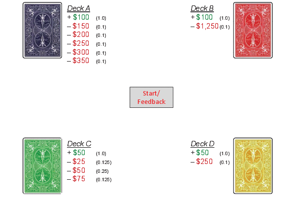
characteristics (see Figure 1). Typically, two decks (hereafter A and
B) are considered “bad” decks, offering high rewards and high
punishments that result in a net loss, whereas two other decks (C and
D) are “good” decks with lower rewards but also lower, more
infrequent punishments (Chiu et al., 2008), resulting in a net gain.
Subjects are not presented with these payment contingencies, but
must learn about each deck through self-directed sampling over the
course of 100 trials.
| Figure 1: Stimulus layout with payment contingencies. Each deck had
a guaranteed payment (noted in green) that appeared on every draw;
a penalty occurred on only some draws (noted in red, with
associated probability). “Start/Feedback” button never actually
appeared on screen with the decks—clicking the start button on
the first trial caused the decks to appear and the button to
disappear. In subsequent trials, clicking on a deck caused the
all decks to disappear and the feedback button to appear. After
feedback was presented, the button disappeared and the decks
reappeared automatically. The deck labels, payoffs, and
probability information shown here are illustrative and was not
presented to subjects. |

2 Experimental design
General paradigm.
The application of the response dynamics
methodology simply requires placing choice options in spatially
disparate regions and tracking mouse movements while subjects make
their selection.2 In contrast to previous response
tracking experiments with binary responses proceeding from the
bottom-center of the screen to the upper-left or upper-right corners,
we produced a multi-alternative version by requiring movement from
screen center to one of the four corners (Figure 1).
To select an option (deck), subjects had to move a cursor from the
start position to the deck of their choice and click. In order to
exploit greater degrees of freedom in the motor response (and thus
allow more opportunity for competitive “pull” to be manifest), we
projected the four choice alternatives onto a wall (approximately 3m x
4m) and had subjects use a wireless pointing device (Nintendo’s
Wiimote; see Dale et al., 2008 for more details) from a distance of
approximately 3m. After clicking on the selected deck, a “Feedback”
box appeared in the start position. To see the outcome of their
selection, subjects had to click on the “Feedback” box, and in
doing so return the cursor to the center start position for the next
trial. Upon clicking, the chosen deck’s outcome was displayed, after
which the reappearance of the decks for the next trial occurred
automatically after a 1-second delay. This implementation ensured
that feedback-related movement was not incorporated into the tracked
response movement of the subsequent trial.
Subjects.
Undergraduates enrolled in introductory
psychology courses were able to sign up for this experiment (among
many) online. Forty-nine undergraduates participated in the study with
five subjects unable to complete the experiment due to computer
failure, producing N = 44 for analyses below. For their participation,
individuals received course credit and a performance contingent
payment, as described below.
Stimuli.
The stimuli in this experiment utilized the
payouts and set order from the traditional IGT (Bechara et al., 1994;
see Figure 1). Over every 10 draws, Decks A and B had an expected
value of -$250 whereas Decks C and D had an expected value of $250.
Unlike the original IGT stimuli where decks were exhausted after 40
draws, subjects had unlimited draws from each deck.
Methods.
After informed consent and a “participation
pledge” to promote investment in the task, subjects received
instruction on the task and payment protocol. Subjects were told
that they would begin the task with an “endowment” of $2000 ($4 in
real money at an exchange rate of $500 to $1) and that their deck
selections during the task could either add to or subtract from this
amount. Subjects were shown animated example trials and completed
one example trial (without feedback) prior to beginning the main task.
Each subject made 100 deck selections, after which they were paid
their adjusted winnings. Decks were always located in the four
corners of the display, yet the locations of the specific decks were
counterbalanced across subjects using four orders (with the
original order in Figure 1 either rotated 180°, or
flipped, or both). We recorded the (x,y)-position of the
cursor at a rate of 100Hz. Importantly, subjects were not told
this nor given special instructions regarding movement of the pointing
device.
| Table 1: Metrics of response dynamics |
| Measure | Explanation | Example article |
| Area under the curve (AUC) | Geometric area falling between the trajectory and a direct path | Freeman & Ambady (2010) |
| Average absolute deviation (AAD) | Mean absolute deviation from a direct path | Freeman & Ambady (2010) |
| Derivative measures | Velocity and acceleration of response trajectory | Wojnowicz et al.,
(2009) |
| XYdist | Total x,y distance traveled in response trajectory | Duran et al.,
(2010) |
| Maximum absolute deviation (MAD) | Maximum absolute deviation from a direct path | McKinstry et al.,
(2008) |
| Xflips | Number of directional changes along the x-axis | Duran et al.,
(2010) |
3 Analyses/Results
The richness of the data provided by online response tracking combined
with the complexity of the IGT creates an overabundance of possible
analyses. For cogency and due to space constraints, we will provide a
few analyses that exemplify the benefits of collecting continuous
response data, but are by no means exhaustive (see Table 1). For more
examples and in depth analyses, we refer the reader to previously
published work using this method (e.g., Spivey, et al. 2005; Dale, et
al., 2007; Duran, et al., 2010; and Freeman & Ambady, 2010).
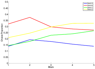
| Figure 2: Choice proportion of each deck
across all blocks |

Aggregate measures.
In order to lend greater structure to
these data, we have divided up subject responses into 5 blocks of
20 trials each. Subjects’ choice patterns across these blocks
provided an initial check on the validity of our version of the IGT.
The general trend (Figure 2) replicates classic findings (e.g.,
Bechara et al., 1994) on the IGT in that choice of the “good” decks
increases throughout the experiment whereas choice of the “bad”
decks decreases. It is interesting to note that although choice of
Deck B (the high variability “bad” deck) decreases throughout the
experiment, it remains relatively high. This paradoxical preference
for Deck B has been noted elsewhere (e.g., Rodríguez-Sánchez et
al., 2005; Wilder et al., 2008; or see Dunn et al., 2006 for a broad
review). Using the metrics facilitated by continuous response
tracking, we can explore this tendency in more detail.
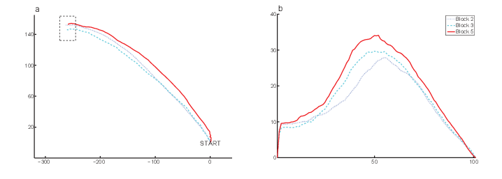
| Figure 3: Time-normalized response profiles for Deck B. (a) Aggregate response
trajectories across subjects for blocks 2, 3, and 5. Locations of
start and response deck are approximate. All responses have been
flipped to upper left in order to collapse across counterbalance
orders. (b) Aggregate response deviation profiles (in pixels) across
subjects for blocks 2, 3, and 5 for each of the 101-time bins
(x-axis). |

The most illustrative descriptive measure of response dynamics is
typically the aggregate response trajectory. The inferential logic is
that as the competitive “pull” from non-chosen options increases, it
is reflected in increased curvature of the response trajectory. Thus,
as one learns about the payment contingencies for each deck, the
“pull” from the bad decks should decrease, resulting in more direct
choices of good decks. Here we present aggregate Deck B trajectories
from three blocks in order to illustrate this traditional response
dynamics presentation (Figure 3a). The data from early (2), middle
(3) and late (5) blocks illustrate changes in this competition (or
reluctance) over the course of the task and roughly correspond to
changes in choice proportions. We produced these trajectories by
time-normalizing each trial with a Deck B selection into 101 time bins
(as done by Spivey et al., 2005) and aggregating within and across
subjects. These time-normalized response trajectories were
reformatted to coincide with Deck B positioned in the upper-left
regardless of its actual physical location (to collapse across
counterbalance conditions). In all previous applications of this
paradigm, which used binary choice, there was only an attraction to
one non-chosen option on each trial (i.e., to the upper right of
Figure 3a). This single competing attractor enabled aggregation
across all trials and subsequent significance testing at each of the
101 time-bins via t-tests (e.g., Spivey et al., 2005), as is typically
done on these trajectories. However, in the multi-alternative IGT task
here, each of three non-chosen decks could exert an attractive
influence in different directions (e.g., to the lower-left).
For clarity, we present in Figure 3a only trials with curvature to the
upper right (after “fixing” counterbalanced physical
location).3 The aggregate
response trajectories for trials with curvature to the lower left show
a similar pattern but are not included. Figure 3b provides similar
information in a manner that allows us to retain all directional
attractors (i.e., include those trajectories that were not plotted in
Figure 3a). Specifically, we computed across time bins the absolute
deviations (from a straight line) in either direction for
each Deck B trajectory for each subject, and then aggregated them.
Relative to the curvature in Block 2 (dotted line, N = 330 trials), in
Block 3 (dashed line; N = 261 trials) subjects have experienced
mainly large gains from the deck and are therefore proceeding more
directly to it (lower deviations). By Block 5 (solid line, N = 238),
however, subjects have experienced many large punishments, making
the decision to select Deck B increasingly difficult as evidenced by
the wider path (greater absolute deviations from a direct path) taken
during this block.
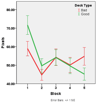
| Figure 4: Mean maximum absolute deviation from direct path. Lines
represent bad decks (A and B; red) and good decks (C and D;
green). After the globally high deviations associated with the
exploratory activity in the first block, maximum absolute
deviation (MAD) generally increases over blocks for selections
from the bad decks, whereas it decreases for selections from the
good decks. |

Individual measures.
The trajectory plots above are
aggregated across subjects due to high individual variability, but
it is important to analyze individual subject data as well (Estes,
1956; Estes & Maddox, 2005) to ensure the aggregate trajectories do
not represent some “virtual subject” who does not truly exist in
the data. In the response dynamics literature, multiple measures have
been considered. Here we utilize individual measures of maximum
absolute deviation from a straight path (MAD), which most closely
correspond to the aggregate data above (Figure 3b). We chose MAD
because it highlights differences in the “heart” of each trajectory,
and is not diluted by the start and end points held in common by all
trajectories. For each individual, we computed the MAD for each deck
type: bad (A and B) and good (C and D). A repeated measures ANOVA
revealed a main effect of block F(4,156) = 13.15, p
< .01, and a marginally significant interaction effect
between block and deck F(4, 156) = 2.22, p = .07. Figure 4
shows that across blocks, MAD decreases for the good decks but
increases for the bad decks. As before, this is interpreted as a
decrease across blocks in competition from the bad decks when
selecting the good decks (decreased reluctance), but an increase in
the competition from the good decks on the bad decks (increased
reluctance).
Outcome-based measures.
Finally, we thought that the
response dynamics might be especially sensitive to the effects of
winning or losing on a deck. For each subject and deck, MAD was
calculated separately for two types of trials: (a) trajectories
towards a deck when the previous selection from that same deck
produced a loss; and (b) trajectories when the previous selection
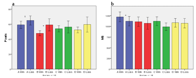
produced a gain.4 Figure 5 shows the
MAD for each deck on trials following that deck’s wins or losses. As
expected, deck selections following a loss have greater deviation
(i.e., involve greater hesitation or conflict) than those following
gains, although this effect was marginally significant, F(1,29) =
3.02, p = 0.09. Planned comparisons show a significant
effect (p < .05) for Deck B and a marginally
significant effect (p < .10) for the other bad
deck, Deck A. A possible critique is that response-tracking metrics
merely reframe information from more traditional measures, like
response time (RT). To address this, we performed the same analyses
on response times for each deck following either losses or wins.
Surprisingly, Figure 5b shows the opposite and counterintuitive
pattern, with selections following a loss happening faster
than those following a gain. Again, the main effect of outcome was
only marginally significant, F(1,29) = 3.20, p = 0.08, and
only the effect for Deck A was significant (p <
.05). Performing these analyses on log-transformed RTs produced
similar conclusions.
| Figure 5: Mean maximum absolute deviation (a) and response time (b)
for each deck by outcome. Selections were grouped by deck choice
and then by previous outcome experienced on that deck. * p
< .05. †p < .10. |

4 Discussion
Our results illustrate the potential of the response dynamics
methodology in its first application to a multi-alternative choice
task, the IGT. Our observed choice proportions are in line with
previous IGT results: as the experiment proceeded, subjects increased
selections from the good decks and decreased selections from the bad
decks. Interestingly, and in line with some previous data,
subjects continued to draw from Deck B somewhat frequently, even
though this frequency decreased over time. Although there was little
change in the choice proportion of Deck B between blocks 3 and 5,
time-normalized deviation profiles indicate that selections from Deck
B were subject to the most competition from other decks during the
final block (Figure 3)—a finding that cannot be inferred from choice
proportions alone. Thus, although we demonstrate continued preference
towards Deck B, the increased curvature on these trajectories
indicates some degree of learning on the task, although determining
whether this learning is motivated by “somatic markers” (Bechara, et
al., 1997; but see Maia & McClelland, 2004 a,b) is beyond the scope
of this experiment. An interesting follow-up question will be whether
trajectories between patient and normal populations differ. If
patients are truly unable to appreciate the impact of large infrequent
penalties, they should not show increases in curvature when drawing
from the bad decks.
Aside from simply exploring Deck B responses more fully, we also
demonstrated general capabilities of this methodology by expanding on
typical IGT analyses. Unique analyses provided by response dynamics
suggest greater competition from bad decks when choosing good decks
early on (Block 2 in Figure 4), perhaps resulting from a reluctance to
leave the large payouts of the bad decks. However, by the end of the
task (Block 5 in Figure 4), subjects have generally learned the
payoff contingencies and thus show greater reluctance when selecting
bad decks rather than good ones. Finally, these inferences can also be
related to the experienced payoffs, which differed across subjects,
blocks, and trials, and thus may dilute the aggregated effects. In
particular, we separately analyzed trajectories following either a loss
or a win and found that, especially for bad deck draws, there was
greater competition after experiencing their losses relative to their
gains (Figure 5a). Importantly, this pattern of results was markedly
different than measures of RT, which showed a decrease
following losses (Figure 5b). Thus, we conclude that metrics afforded
by response dynamics provide a window into cognitive processes that is
unique from more traditional measures.
While these data provided a brief example of how response dynamics can
be fruitfully applied to a common decision task, our excitement about
this methodology stems largely from its potential to aid in the
resolution of theoretical disputes. Below, we provide a brief
“roadmap” for how the continuous data provided by response dynamics
could distinguish between three different classes of models:
one-reason decision making (e.g., Gigerenzer & Goldstein, 1999),
so-called default-interventionist (Evans, 2008) dual-systems models
(e.g., Kahneman & Frederick, 2002), and sequential sampling models
(e.g., Busemeyer & Townsend, 1993; Diederich, 1997). From each of
these models, we can derive very specific predictions about the form
of response trajectories.
Strong versions of one-reason decision-making models (e.g., Gigerenzer
& Goldstein, 1999) would predict noncommittal trajectories that
suddenly and sharply give way to an expression of preference. This
sudden and sharp development of preference would be represented by
velocity profiles with late spikes, and would not predict any online
preference reversals. Contrarily, dual-systems models would predict
these online preference reversals when response options place
intuitive (system 1) and deliberative (system 2) systems at odds with
one another. Of particular interest would be choices of the option
preferred by system 2. Because system 1 is thought to be faster, on
these trials trajectories should first proceed towards the system 1
option, before the deliberative system “overrides” this impulse
causing an online preference reversal towards the deliberative option.
Although these online preference reversals would preclude one-reason
decision-making models, they would not necessarily distinguish between
dual-systems and sequential sampling models. In order to further
break apart these competing models, response dynamics could be paired
with eye-tracking to see whether these reversals are the product of
changes in attention. Sequential sampling models would predict that
changes in trajectory direction would be directly tied to changes in
attention (e.g., Diederich, 1997), whereas dual-systems accounts would
not necessarily predict such a systematic relationship between
attention and preference.
In summary, we showed that response dynamics provides useful information
unique from traditional measures, and provided a broad framework
outlining how response dynamics could distinguish between competing
models. Because mouse tracking has been shown to provide a real-time
measure of cognitive processing (Freeman et al., 2011), we thus
conclude that it can be widely applied to directly test process models
of decision making and hope the current demonstration can help open the
door to future work that will continue to do so.
References
Bechara, A., Damasio, A. R., Damasio, H., & Anderson, S. W. (1994).
Insensitivity to future consequences following damage to human
prefrontal cortex. Cognition, 50, 7–15.
Bechara, A., Damasio, H., Tranel, D., & Damasio, A. R. (1997).
Deciding advantageously before knowing the advantageous strategy.
Science, 275, 1293–1295.
Bergert, F. B., & Nosofsky, R. M. (2007). A response-time approach to
comparing generalized rational and take-the-best models of decision
making. Journal of Experimental Psychology, 33, 107–129.
Busemeyer, J. R., Jessup, R. K., Johnson, J. G., & Townsend, J. T.
(2006). Building bridges between neural models and complex decision
making behaviour. Neural Networks, 19, 1047–1058.
Busemeyer, J. R., & Johnson, J. G. (2008). Microprocess models of
decision making. In R. Sun (Ed.), Cambridge Handbook of
Computational Psychology, 302–321. Cambridge University Press.
Busemeyer, J. R., & Townsend, J. T. (1993). Decision field theory: A
dynamic-cognitive approach to decision making in an uncertain
environment. Psychological Review, 100, 432–459.
Chiu, Y., Lin, C. H., Huang, J. T., Lin, S., Lee, P. L., & Hsieh, J. C.
(2008). Immediate gain is long-term loss: Are there foresighted
decision makers in the Iowa Gambling Task? Behavioral and
Brain Functions, 4(13).
Busemeyer, J. R. & Johnson, J. G. (2004). Computational models of
decision making. In D. Koehler & N. Harvey (Eds.), Blackwell
Handbook of Judgment and Decision Making. Oxford, UK: Blackwell
Publishing Co. 133–154.
Dale, R., Kehoe, C. E. & Spivey, M. J. (2007). Graded motor responses
in the time course of categorizing atypical exemplars. Memory
and Cognition, 35, 15–28.
Dale, R., Roche, J., Snyder, K., McCall, R. (2008). Exploring action
dynamics as an index of paired-associate learning. PLoS ONE
3(3): e1728.
Dunn, B. D., Dalgleish, T., & Lawrence, A. D. (2006). The somatic
marker hypothesis: A critical evaluation. Neuroscience and
Biobehavioral Reviews, 30, 239–271.
Duran, N. D., Dale, R., & McNamara, D. (2010). The action dynamics of
overcoming the truth. Psychonomic Bulletin & Review, 17,
486–491.
Estes, W. K. (1956). The problem of inference from curves based on
group data. Psychological Bulletin, 53, 134–140.
Estes, W. K., & Maddox, W. T. (2005). Risks of drawing inferences
about cognitive processes from model fits to individual versus average
performance. Psychonomic Bulletin and Review, 12, 403–408.
Evans, J. St. B. T. (2008). Dual-processing accounts of reasoning,
judgment and social cognition. Annual Review of Psychology,
59, 255–278.
Franco-Watkins, A. M., & Johnson, J. G. (2011). Decision
moving window: Using interactive eye tracking to examine decision
processes. Judgment and Decision Making, 6, 740–748.
Freeman, J. B., & Ambady, N. (2010). MouseTracker: Software for
studying real-time mental processing using a computer mouse-tracking
method. Behavior Research Methods, 42, 226–241.
Freeman, J. B., Dale, R., & Farmer, T. A. (2011). Hand in motion
reveals mind in motion. Frontiers in Psychology, 2, 59.
Freeman, J. B., Pauker, K., Apfelbaum, E. P., & Ambady, N. (2010).
Continuous dynamics in the real-time perception of race.
Journal of Experimental Social Psychology, 46,
179–185.
Gigerenzer, G., & Goldstein, D. G. (1999). Betting on one good reason:
The Take The Best heuristic. In Gigerenzer, G., Todd, P.M., & the ABC
Research Group, Simple Heuristics That Make Us Smart. New
York: Oxford University Press.
Glöckner, A. (2009). Investigating intuitive and deliberate processes
statistically: The multiple-measure maximum likelihood classification
method. Judgment and Decision Making, 4, 186–199.
Hilbig, B. E. (2008). One-reason decision making in risky choice? A
closer look at the priority heuristic. Judgment and Decision
Making, 3, 457–462.
Kahneman, D., & Frederick, S. (2002). Representativeness
revisited: Attribute substitution in intuitive judgment. In T.
Gilovich, D. Griffin, & D. Kahneman (Eds.), Heuristics
and biases: The psychology of intuitive judgment, pp. 49–81.
New York. Cambridge University Press.
Koop, G. J., & Johnson, J. G. (2011). Beyond process tracing:
The response dynamics of preferential choice. Unpublished manuscript.
Johnson, J. G., & Busemeyer, J. R. (2005). A dynamic, stochastic,
computational model of preference reversal phenomena.
Psychological Review, 112, 841–861.
Maia, T. V., & McClelland, J. L. (2004a. A reexamination of the
evidence for the somatic marker hypothesis: What participants really
know in the Iowa gambling task. Proceedings of the National
Academy of Sciences U.S.A., 101, 16075–16080.
Maia, T. V., & McClelland, J. L. (2004b). The somatic marker
hypothesis: still many questions but no answers. Trends in
Cognitive Sciences, 9, 162–164.
McKinstry, C., Dale, R., & Spivey, M. J. (2008). Action dynamics
reveal parallel competition in decision making. Psychological
Science, 19, 22–24.
Payne, J. W. (1976). Task complexity and contingent processing in
decision-making—Information search and protocol analysis.
Organizational Behavior and Human Performance, 16, 366–387.
Payne, J. W., Bettman, J. R., & Johnson, E. J. (1988). Adaptive
strategy selection in decision making. Journal of Experimental
Psychology: Learning, Memory, and Cognition, 14, 534–552.
Riedl, R., Brandstätter, E., & Roithmayr, F. (2008). Identifying
decision strategies: A process- and outcome-based classification
method. Behavior Research Methods, 40, 795–807.
Rodríguez-Sánchez, J. M., Crespo-Facorro, B., Iglesias, R. P.,
Bosch, C. G., Álvarez, M., Llorca, J., & Vázquez-Barquero, J. L.
(2005). Prefrontal functions in stabilized first-episode patients with
schizophrenia spectrum disorders: A dissociation between dorsolateral
and orbitofrontal functioning. Schizophrenia Research, 77,
279–288.
Russo, J. E., & Rosen, L. D. (1975). An eye fixation analysis of
multialternative choice. Memory & Cognition, 3, 267–276.
Schulte-Mecklenbeck, M., Kühberger, A., & Ranyard, R. (2010).
A Handbook of Process Tracing Methods for Decision Research: A
Critical Review and User’s Guide. New York: Taylor &
Francis.
Song, J.H., & Nakayama, K. (2009). Hidden cognitive states revealed in
choice reaching tasks. Trends in Cognitive Sciences, 13,
360–366
Spivey, M. J. (2007). The continuity of mind. New York:
Oxford University Press.
Spivey, M. J., & Dale, R. (2006). Continuous dynamics in real-time
cognition. Current Directions in Psychological Science, 15,
207–211.
Spivey, M. J., Grosjean, M., & Knoblich, G. (2005). Continuous
attraction toward phonological competitors. Proceedings of the
National Academy of Sciences of the United States of America, 102,
10393–10398.
Wedel, M., & Pieters, F. G. M. (2000). Eye fixations on advertisements
and memory for brands: a model and findings. Marketing
Science, 19, 297–312.
Wilder, K. E., Weinberger, D. R., & Goldberg, T. E. (1998). Operant
conditioning and the orbitofrontal cortex in schizophrenia patients:
Unexpected evidence for intact functioning. Schizophrenia
Research, 30, 169–174.
Wojnowicz, M. T., Ferguson, M.J., Dale, R., & Spivey, M. J. (2009).
The self-organization of explicit attitudes. Psychological
Science, 20, 1428–1435.
This document was translated from LATEX by
HEVEA.
