Judgment and Decision Making, vol. 6, no. 3, April 2011, pp. 211-221

Fiedler et al. (2009), reviewed evidence for the utilization of a contingency inference strategy termed pseudocontingencies (PCs). In PCs, the more frequent levels (and, by implication, the less frequent levels) are assumed to be associated. PCs have been obtained using a wide range of task settings and dependent measures. Yet, the readiness with which decision makers rely on PCs is poorly understood. A computer simulation explored two potential sources of subjective validity of PCs. First, PCs are shown to perform above chance level when the task is to infer the sign of moderate to strong population contingencies from a sample of observations. Second, contingency inferences based on PCs and inferences based on cell frequencies are shown to partially agree across samples. Intriguingly, this criterion and convergent validity are by-products of random sampling error, highlighting the inductive nature of contingency inferences.

Keywords: sampling distribution, operant learning, predictions.

1  Introduction

Accurate contingency assessment is a prerequisite to “explain the past, control the present and predict the future” (Crocker, 1981, p. 272). From an adaptive cognition perspective, assessing contingencies amounts to inferring the relationship between two variables in a population from a sample of observations drawn from that population (Lopes, 1982). If the task was to evaluate the relation between drinking one of two beverages, say red wine or beer, and developing a migraine or not, the contingency may be inferred from recalling instances of wine and beer consumption followed or not followed by a migraine.

Epistemologically, then, the contingency in a sample, or more precisely the specific contingency index used by the decision maker, is used as a proxy for the contingency in the general population of instances. For example, to the degree that for the last 10 instances of alcohol consumption the proportion of developing a migraine was higher after red wine than after beer, one might conclude that in general red wine is more conductive of migraine than beer. Not only for the ΔP index in this example but for most contingency indices this inference seems unproblematic, as the sign and size of the sample value are unbiased estimates of the population value (for an exception see Kareev, 2000).

What might be more problematic is the quality grade of the information required. Virtually all traditional contingency indices require information about joint occurrences. In other words, for every instance in a sample it is necessary to know the levels of both variables. In the example, for every consumption instance one needs to be sure whether red wine or beer had been consumed and whether it was followed by a migraine or not. However, due to several factors, e.g. a delay between observing the variables or a large amount of variables to be considered, information about joint occurrences might not be available at the time of judgment, preventing the use of the common contingency indices.

In the remainder, we will discuss the validity of an alternative strategy for contingency inferences that is applicable even under such impoverished conditions: Pseudocontingencies. PCs denote using the skew (greater numbers of one level than the other in the case of dichotomous variables) in the sample base rates of a pair of variables to infer a contingency. It is obvious that by using base rates, PCs do not require information about joint occurrences. However, because base rates are largely independent from contingencies, it is less obvious why PCs should be used at all. While independence is true descriptively at the population level, we will show that random sampling error necessarily causes population contingencies to translate into skewed sample base rates. Intriguingly, these sample base rates, skewed by the sampling process, enable PCs to successfully indicate (moderate to strong) population contingencies. As another consequence, strategies that rely on joint occurrences mostly agree with the PCs’ predictions across samples. Thus, in addition to being more economical than other indices, we argue that PCs are subjectively valid because of their validity to infer the criterion, the population contingency, and because of their convergent validity with other strategies.

2  PCs: inferring contingencies from base rates

Specifically, PCs link the more frequent levels and, by implication, the less frequent levels for a pair of variables to one another. For instance, if in a given sample, remembered consumption instances of red wine were more frequent than those involving beer and given that the majority of all instances was followed by a migraine, a PC would link red wine consumption to migraine.

---

Table 1: Example of a standard 2 x 2 contingency table.

		M(igraine)
		Yes	No
D(rink)	Red wine	a	b	Dred wine
	Beer	c	d	Dbeer
		Myes	Mno

---

Notably, PCs completely ignore information about joint occurrences—relying solely on base rates (see below for a formal definition). In terms of a standard 2 x 2 frequency table such as the one depicted in Table 1, PC inferences do not build on cell frequencies commonly denoted by the letters a, b, c, and d (e.g., red wine consumption followed by a migraine would correspond to the a-Cell)—but on the marginal frequencies or base rates (e.g., of drinks and migraine symptoms separately) here denoted as D_red wine, D_beer, M_yes, and M_no. Formally speaking, PCs can be defined as the sign of the product of base rate differences:

Thus, PCs imply a positive contingency when the base rates of the target variables are skewed in the same direction and a negative contingency when the base rates are skewed in opposite directions. In other words, utilizing a PC relies on nothing more than the similarity of two attribute levels in terms of their frequency: if both levels can be termed frequent or infrequent, positive contingency inferences result. If levels are dissimilar in terms of being frequent or infrequent, negative contingencies are inferred. If frequent or infrequent do not apply to either one or both of the attribute levels, the inference is zero. Thus, irrespective of the size of the base-rate deviation, the PC strategy relies only on base-rate information to infer the sign of a contingency.

This stands in contrast to contingency indices that have been proposed to describe human contingency judgments, all of which exclusively rely on cell frequencies to describe contingencies. For example, a normative contingency index also used to describe human contingency assessments is ΔP (Allan, 1993; Allan & Jenkins, 1983; Cheng & Novick, 1992; Jenkins & Ward, 1965; Ward & Jenkins, 1965). ΔP compares the proportions of observations of one level on one attribute (e.g., the proportion of migraine instances), for both levels on the other attribute (e.g., having consumed red wine or beer). This is formally expressed as Δ P = a/(a+b) − c/(c+d). One important aspect this index shares with other normative contingency indices is that base rates do not determine the sign of contingencies. Even if red wine was more frequent than beer, and migraine was more frequently present than absent, the proportion of developing migraine can still be higher after beer consumption. As a consequence, PCs seem unwarranted, because—descriptively—marginal frequencies do not determine the sign of contingencies.

Nevertheless evidence has accumulated for a wide range of task settings and dependent measures that people draw on PCs when making contingency inferences based on samples of observations (beginning with Hamilton & Gifford, 1976; for a review see Fiedler, Freytag, & Meiser, 2009). For example, in a series of studies, participants were to infer the relation between two different diets in a hospital (vegetarian or prebiotic) and the symptom level (high or low) after fixed trial by trial sampling of information from 96 patients (Fiedler & Freytag, 2004). In this demonstration, one diet and one symptom level were more frequent than the respective others, both at a ratio of three to one. When information about diets was presented separately from information about symptoms, so that cell-frequency information was unavailable and no contingency was defined, inferences still linked the frequent level of the diet to the frequent level of the symptoms. For example, for new patients, participants predicted the rare levels of one variable to a higher degree when the rare as compared to the frequent level of the other variable was known to be present.

Another illustrative example comes from a study on group impression formation. Eder and his collaborators (Eder, Fiedler, & Eder-Hamm, in press) found a standard illusory correlation effect in that a majority group was evaluated more in line with the frequently presented valence than a minority group. Different from most other studies on illusory correlations, they also found this relation when group members and positive or negative behaviors were presented separately so that, again, cell frequency information and a contingency were not defined (for evidence from a similar procedure, see McGarty, Haslam, Turner, & Oakes, 1993). These experiments eliciting contingency judgments without providing cell frequencies offer the most direct evidence for PCs as they cannot be explained by the use of other cell-frequency based strategies.

Additionally, several studies found evidence for judgments following the PC strategy even when cell frequency information was readily available. These studies pitted the predictions of cell frequency based indices, usually ΔP, against the PC strategy predictions. For example, when free to sample in a multivariate environment consisting of four demographic indicators, participants’ subsequent predictions linked the variables that were jointly frequent or infrequent irrespective of their contingency (0 or .3 in the opposite direction). Moreover they did not link variables that were not jointly skewed but linked by a contingency of .3 (Fiedler, 2010; see also Meiser & Hewstone, 2004). In yet another demonstration, the tendency to associate frequent outcomes with frequent signals irrespective of a zero contingency between them persisted in an operant matching-to-sample paradigm when correct and false predictions had monetary consequences (Kutzner, Freytag, Vogel, & Fiedler, 2008).

The robustness of the phenomenon notwithstanding, the very reasons for the subjective validity of PCs are as yet poorly understood. If anything, previous treatments of the issue analyzed the task conditions under which PCs were observed (Fiedler et al., 2009). As already mentioned, it has been argued that, on one hand, the environment may often fail to render cell frequencies available in the first place. With no cell frequencies available, people may resort to using the PC strategy derived from easily available base rates (Hasher & Zacks, 1984). On the other hand, it has been argued that the environment may simply be too complex to allow for the utilization of strategies relying on cell frequency information. For a set of no more than four dichotomous variables, as in the experiment by Fiedler (2010), keeping track of the joint occurrence of all pairs of variables requires no less than the monitoring of 4*(4–1)/2 = 6 2 x 2 tables, surmounting in 24 cell frequencies. Given the limitations of human information processing, decision makers might resort to using base rates as the flood of information coming from the environment may create a situation in which the cell frequencies are unavailable at the time of judgment, due to insufficient cognitive capacity.

As compelling as these arguments may appear, they do not explain why decision makers over-generalize the usage of PCs to conditions of reduced complexity and complete information. In an attempt to answer this question we propose that PCs are used because they are perceived to be valid: valid in order to infer population contingencies and, at the same time, valid to maintain coherence with other strategies employed to achieve the same end.

3  Criterion validity

The subjective validity of the PC strategy might stem from its validity for predicting the criterion, the sign of the population contingency. Even if, by definition, the population contingency cannot be directly assessed to serve as criterion, it should influence learning from feedback. If contingency inferences are used to make predictions about future events, the rate of reinforcing feedback will be higher when the direction of the contingency at the population level was correctly inferred. For example, when developing a migraine was identified to be contingent on red wine rather than beer in the sample, substituting red wine with beer would be an intuitive avenue in trying to reduce the frequency of migraines. The success rate of such enterprises, though dependent on many additional factors, will critically depend on whether the contingency inference was correct in the first place. Thus, even though not directly accessible, the population contingency might serve as a criterion for validity of PCs via feedback learning. An estimate of the criterion validity of the PC strategy would be the accuracy with which the sign of a population contingency can be inferred from base rate information in the sample. To the degree that the PC strategy should perform well the decision maker should learn to use it.

---

Table 2: Frequency tables for samples of n = 10 observations drawn from a population with a perfect contingency between the evenly distributed attributes mutation and disease.

		Sample 1			Sample 2			Sample 3
		Migraine			Migraine			Migraine
		Yes	No		Yes	No		Yes	No
Drink	Red wine	5	0	5	6	0	6	2	0	2
	Beer	0	5	5	0	4	4	0	8	8
		5	5	10	6	4	10	2	8	10

---

4  Convergent validity

Another possible source for the PC’s subjective validity might be its convergence with other contingency inference strategies derived from cell frequencies. This form of convergent validity builds on what is directly accessible to the decision maker, the sample based predictions of different strategies. In other words, even though cell frequencies and base rates are different sources of information, the conclusions separately derived from either one might nonetheless coincide. For example, imagine that an attempt to recall consumption-migraine instances not only produces more red wine than beer and more migraine than non-migraine recollections—being conducive to a PC. But also imagine that it produces a large number of recollections when red wine consumptions were followed by a migraine, resulting in a large a-Cell, and less recollections for the other combinations. Although people vary widely in how they weigh cell frequencies (see below), because of the comparatively large a-Cell, this example would probably result in the same contingency inference as the PC strategy, red wine being related to migraine.

More generally, the PC and cell-frequency based strategies should be perceived to converge when (a) the proportion of same sign inferences is high and (b) the cell-frequency based index is, on average, larger in samples indicating a positive as compared to samples indicating a negative PC inference. To the degree that this is the case, a decision maker may be tempted to use the more economical PC strategy as a default, because the effortful utilization of cell frequency information would not seem to yield sufficient additional insights into the correlational structure of the environment.

5  The role of random sampling error

Before turning to the simulation of the PC strategy’s criterion and convergent validity, a thought experiment illustrates how a powerful and omnipresent agent promotes the validity of PCs: random sampling error. For a start, imagine that in the population referred to in our opening example, developing a migraine is perfectly contingent on drinking red wine—and that the base rates for both, drinking wine or beer and developing a migraine or not are 50%. Of course, randomly sampling from such a population will always result in a perfect contingency in the sample because there are, by definition, no instances where beer consumption was followed by a migraine or red wine consumption was not followed by a migraine (see Table 2).

Note that, in sharp contrast to the invariance of the perfect sample contingencies, the base rates in the samples can still vary. When sampling error causes one base rate to deviate from 50% (e.g., with occasionally 6 out of 10 red wine instances), the other base rate necessarily deviates from equality as well (i.e., with 6 out of 10 migraine instances). In the extreme case of a perfect population contingency, a sample-based PC strategy will either incorrectly indicate a zero contingency (see sample 1) or correctly indicate the direction of the population contingency (see sample 2 and sample 3). Repeating the sampling process may thus render the PC strategy predictive—on average—of the sign of the population contingency.

To sum up, we expect sampling error to lead to skewed sample base rates, even when population base rates are not skewed, in a way that causes PC inferences to be accurate (at least for substantial population contingencies) and to converge with contingency inferences derived from cell frequencies.

6  Overview of the simulation

We used a simulation to generalize and quantify the degree to which the PC strategy accurately indicates the direction of varying population contingencies and to assess its convergence with another psychologically plausible cell-frequency based strategy. Because of the central role of the population contingency in interaction with random sampling, we created populations covering the full range of possible contingencies in terms of ΔP and drew random samples of varying sizes. These random samples were used to infer the sign of the population contingency from the base rates according to the PC strategy, as well as from the cell frequencies according to another possibly representative cell-frequency based strategy, the aggregate-model strategy (AGG-model, McKenzie, 1994; Hattori & Oaksford, 2007).

Selecting a specific representative strategy is difficult because people vary widely in which cell-frequency based strategy best describes their contingency inferences (e.g., Shaklee, & Tucker, 1980). However, for several reasons the AGG-model offers a good generic standard to assess the PCs convergent validity. Most importantly, human contingency judgments on average seem to increase most with the a-Cell, only weakly with the d-Cell, and seem to decrease more with the b-Cell than with the c-Cell (for a review see, Lipe, 1990; Wasserman, Dorner, & Kao, 1990). This meta-analytic finding is directly reflected in the AGG-model strategy, formally defined as

In addition to describing a host of empirical evidence on human contingency judgments, the AGG-model correlates highly with other intuitive strategies such as Positive-testing, Sum-of-diagonals or even ΔP, used to characterize the criterion (McKenzie, 1994). Finally, due to its simplicity, the AGG-model is ideally suited for inferring contingencies based on limited samples. In contrast, because ΔP involves division operations, it cannot make predictions when one of the predictor levels was not observed at all reducing its validity for small samples. Therefore, we use the AGG-model strategy as a generic psychologically plausible reference strategy to evaluate the PC strategy’s convergent validity.

Specifically, the simulation was designed to capture a situation akin to our example in which a decision maker wishes to infer the direction of a population contingency from a sample of observations gathered over time. For this first demonstration we additionally assumed that the decision maker had no influence on the random sampling process. To capture different degrees of sampling or experience with the contingency at hand, we included different sample sizes, a snapshot of seven observations conveniently stored in working memory and a large sample of 100 observations.

We expected that the criterion validity of the PC strategy would increase with increasing population contingencies and that it would perform above chance at least for strong population contingencies. For the AGG-model, we expected a similar pattern because a stronger population contingency is a stronger signal competing with the sampling error (Lopes, 1982). On average, we expected the AGG-model strategy to perform better than the PC strategy, as it uses all available information, and we expected accuracy to increase with sample size.

6.0.1  Method

We created 11 populations with ΔP values ranging from 0 to 1.0 by defining cell-frequency values (see Table 3).¹ We will discuss the strategies’ accuracy and convergence conditional on the level of contingency in the population. Doing so, we do not make assumptions about the distribution of contingencies in the real world. Initially the populations were not characterized by any skew of the base rates to demonstrate how the skew in the samples arises from sampling error alone. The case of skewed population base rates is addressed in the General discussion.

Having in mind the migraine example in which the cell frequencies result from searching a certain time span in memory, we assumed a Poisson process to generate the random samples. Thus, for every population we generated 10,000 random samples assuming an independent Poisson process for each cell with mean values equal to the cell frequencies of the populations. Because using the cell frequencies in Table 3 results in samples of seven observations on average, we repeated the sampling process after multiplying the mean values by 100/7, resulting in samples of 100 observations on average.

---

Table 3: Cell-frequency values in the 11 populations used in the simulation

ΔP	0	.1	.2	.3	.4	.5	.6	.7	.8	.9	1.0
a	1.750	1.925	2.100	2.275	2.450	2.625	2.800	2.975	3.150	3.325	3.500
b	1.750	1.575	1.400	1.225	1.050	0.875	0.700	0.525	0.350	0.175	0.000
c	1.750	1.575	1.400	1.225	1.050	0.875	0.700	0.525	0.350	0.175	0.000
d	1.750	1.925	2.100	2.275	2.450	2.625	2.800	2.975	3.150	3.325	3.500

---

For every sample, we computed the proportion of predictions for a negative, zero or positive contingency, of the PC and the AGG-model strategies. Across samples, we defined accuracy as the strategies’ proportion of correct sign inferences (i.e., the proportion of positive sign inferences for the positive contingency populations). We will refer to chance as guessing either a positive or a negative contingency, which results in a chance accuracy of 50%. Even though plausible for some tasks, we excluded guessing a zero contingency, which would have lowered chance accuracy to 33%, to have a more conservative test of the strategies’ average accuracies.

6.0.2  Results and discussion

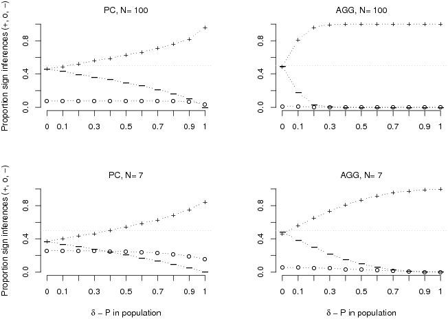
Criterion validity. Figure 1 shows the specific sign inferences, positive (+), zero (0) and negative (–), of the PC and the AGG-model strategy. As hypothesized, the accuracy of both strategies increases with the population contingency and with sample size. Notably, the PC strategy (left hand panels in Figure 1) reaches above-chance accuracy based on the large sample whenever population contingencies are stronger than .1 and, based on the small sample, whenever population contingencies are stronger than .4. Given that base rates in the population were evenly distributed, this effect is entirely due to random sampling error.

---

Figure 1: Proportions of positive (+), zero (0) or negative (-) sign inferences of the population contingency derived from the PC and the AGG-model strategy are depicted as a function of population contingency and sample size. For each population contingency, estimates are based on 10,000 random samples generated by a Poisson process.

---

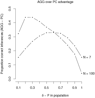
As to the AGG-model strategy (right hand panels in Figure 1), accuracy is above chance for all population contingencies larger than zero and depends on the same factors as the accuracy of the PC strategy, weaker population contingencies and smaller samples causing performance to drop. As expected, the AGG-model strategy in comparison performs better than the PC strategy. This comes to no surprise as it uses more information. Figure 2 illustrates that this advantage is most pronounced for the combination of larger samples and smaller population contingencies.

Another noteworthy aspect is the strategies’ inability to infer a zero population contingency. As implemented, both strategies are systematically biased towards making α -errors, that is, against indicating zero-contingencies. Changing the strategies by introducing thresholds, for example a minimal skew that has to be sampled in order for the PC strategy to indicate a non-zero contingency, would remove this asymmetry. Even though plausible, we refrain from discussing the additional assumptions needed, as they do not change the fact that both, PC and AGG-model, perform above chance for substantial contingencies.

Taken together, the criterion validity analysis shows that relying on base rates in the form of PCs allows for inferring the sign of population contingencies with above-chance accuracy when population contingencies are substantial. Thus, when cell frequencies are missing or too numerous, the PC strategy might be used due to its validity with respect to the contingencies in population. The PC strategy should become even more attractive when assuming that correctly inferring strong contingencies provides the largest relative pay-off to the decision maker.

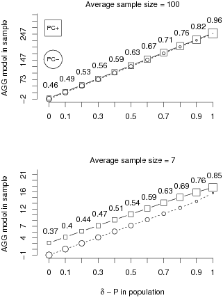
Convergent validity. As a second source of validity we hypothesized that the PC strategy partially converges with other intuitive strategies. Figure 3 shows the convergence between the PC and the AGG-model strategy, by plotting the average AGG-model values for samples implying positive and implying negative PCs (squares and circles, respectively) and the proportions of samples that show positive or negative PCs for each population contingency (indicated by the size of the symbols).

---

Figure 2: Differences in proportion of correct sign inferences of the AGG-model minus the PC strategy are shown as a function of population contingency and sample size. For each population contingency, estimates are based on 10,000 random samples generated by a Poisson process.

---

---

Figure 3: Average AGG-model values are depicted separately for samples with positive (squares) and negative (circles) PCs as a function of the contingency in the population and the sample size. The size of the symbols is proportional to the proportion of the samples in the 10,000 simulation runs per population contingency with the values equal to the proportions of samples indicating a positive PC.

---

Note that, as expected, the AGG-model value is correlated with the ΔP in the population. In addition and crucial to the present argument, we find that the PC and the AGG-model strategy partially converge for all population contingencies and all sample sizes. As evident from relatively larger squares indicating positive PC inferences, the proportion of same sign inferences is above 50% whenever the contingency in the population is above .2 for the large and above .3 for the small sample (see Figure 3 for exact proportions of samples indicating a positive PC). This effect is most pronounced for substantial contingencies where hardly any conflicting predictions emerge.

Complementing the proportion effect, as evident from the location of the lines, we find that samples implying positive PCs are characterized by higher average AGG-model values than samples implying negative PCs across the entire range of population contingencies. Relative to the range of AGG-model values this covariation is more pronounced for the smaller sample. Together, the mean difference and the higher proportion of same-sign samples indicate that there is considerable convergence between the predictions of the PC and the AGG-model strategies especially for substantial population contingencies and small sample sizes.

In sum, the analysis of convergence provides support for the claim that the PC strategy might be subjectively valid because it converges with an intuitive cell-frequency based strategy, the AGG-model, over the entire range of possible population contingencies. Even though not demonstrated here, this generalizes to other psychologically plausible strategies for contingency assessment proposed by McKenzie (1994) that are highly correlated with the AGG-model, including ΔP.

Thus, whenever decision makers are in the position to make contingency inferences based on cell frequencies they can learn about the strategies’ redundancy with the PC strategy. Similar to other cognitive tasks using multiple sources of information, for example depth perception, the redundancy should create vicarious functioning leading to a form of perceived convergent validity and to PCs substituting other strategies when cell frequencies are not available or information is too complex.

7  General discussion

Pseudocontingencies (PCs), relying on base rates to infer contingencies, have been proposed and empirically supported as a simple alternative to cell-frequency based strategies (Fiedler et al., 2009). In essence, the PC strategy predicts a positive contingency between two attributes if two attribute levels are either both frequent or both infrequent. Analogously, the PC strategy predicts the opposite, or a negative contingency, when one attribute level is frequent and the other infrequent, and no contingency when any of the attribute levels is as frequent as the corresponding other level. This is crucially different from other normative or intuitive contingency inference strategies, as all of these strategies need cell-frequency information to arrive at predictions. Even though this novel conception of contingency inferences might seem odd at first sight, it is far from being arbitrary.

Why are PCs used? In the present work, we propose that the PCs’ subjective validity contributes to their usage. We provide evidence for two possible sources of subjective validity: criterion validity with respect to reality when inferring contingencies beyond the given sample, and convergent validity with respect to other intuitive strategies to arrive at contingency inferences in a given sample. In a first analysis we showed that applying the PC strategy allows for inferring the sign of a population contingency with above-chance accuracy when these contingencies are not too small (i.e. larger than .4 for small samples). Thus, in situations where only base rates are available, for example because joint observations of predictors and outcomes were forgotten, the PC strategy seems the only valid strategy to infer contingencies.

Where cell-frequency information is available, we showed that cell frequency based strategies, for example the AGG-model strategy, are even more valid for inferring the sign of a contingency. Therefore one might argue that these other strategies might be used whenever possible (e.g., Rieskamp & Otto, 2006). However, the PC strategy should enjoy an advantage under conditions of limited cognitive resources, as it does not require instances from one variable to be coordinated with those from the other variable, instead relying on the comparison of easily stored cardinal frequencies (Hasher & Zacks, 1984). It should also be hard for a decision maker to distinguish empirically between the validities of both types of strategies because they converge most of the time. As the second analysis reveals, there are few instances, especially for strong contingencies, where the PC and the AGG-model strategies diverge in their predictions. Thus, subjectively the PC strategy might also gain validity in a convergent sense with other intuitive strategies as reference.

Rarity and compensatory sampling. In the present analysis we wanted to emphasize that the validity of the PC strategy arises from sampling error alone. Thus, no PCs were present in the populations and attribute base rates were evenly distributed throughout. Similarly, in our opening example we suggested that neither of the attribute levels, consuming red wine or beer and developing a migraine or not, could be regarded as rare as compared to the respective other level. Naturally, in reality the base rates on the level of the population might depart from even distributions. For example, drinking red wine might be less frequent than drinking beer, and developing a migraine might, hopefully, be less frequent than not developing a migraine. In covariation based causal induction it was even suggested that the joint rarity of causes and effects might be the rule rather than the exception (Hattori & Oaksford, 2007; McKenzie & Mikkelsen, 2007). For inferring contingencies between such variables, the criterion and convergent validities of the PC strategy seem restricted as the PC strategy is bound to always yield a positive contingency inference.

Probably true for some cases, rarity only restricts the validity of the PC strategy based on purely opportunistic sampling. However, there is reason to doubt that decision makers sample passively when they have a priori knowledge about the skew of the variables and the ability to control the sampling process. In our example, when knowing that you drink beer more often than red wine, opportunistic sampling would imply ending up with far more recollections of beer-consumption instances. Alternatively, knowing about the prevalence of one’s beer-consumption, one might try harder and go back further in memory to recollect red wine-consumption instances, compensating the skew in the base rate.

Kareev and Fielder (2006) recently provided evidence for this claim. In a free sampling procedure, participants were to search information about clinical problems from stacks of cards that were arranged by their attribute levels. For example, one problem was to assess the relation between the type of hospital and whether or not a patient experienced complications. Importantly, this procedure leaves base rates clearly visible from the size of the respective stacks. Results indicated that the rare attribute levels were severely oversampled, accounting for only 18% of the original information but for 43% in the average participant sample. This tendency to actively compensate by oversampling rare attribute levels, if possible, should reinstate the PCs validity in the “compensated” sample.

To substantiate that under compensatory sampling the PC strategy is again valid for inferring the sign of a population contingency, we slightly modified our simulation.² The populations, still varying in the size of the contingency, were now characterized by a joint skew in the variables of 3 to 1.³ Thus rarity was created that left the rarest joint observations, a-Cell observations, accounting for 6%–25% of the cases depending on the population contingency. Compensatory sampling was implemented by repeating the sampling process 3 times for the rare cells of the predictor variable, that is the a- and b-Cells. 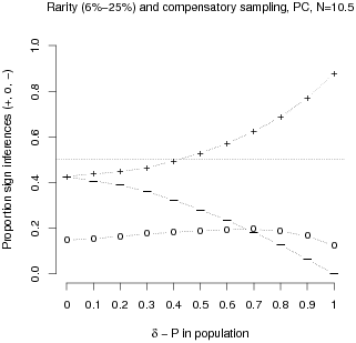The proportion of sign inferences based on these compensated samples are depicted in Figure 4.

---

Figure 4: Proportions of positive (+), zero (0) or negative (-) sign inferences of the population contingency derived from the PC strategy. Both variables have rare attribute levels at a ratio of 3 to 1 with the rarest combination accounting for 6%–25% of the cases, depending on the population’s contingency. For each population contingency, estimates are based on 10,000 samples generated by a Poisson process. For the criterion variable the process was random. For the predictor variable the rare event was oversampled in a compensatory way by a factor 3.

---

The results indicate that the performance of the PC strategy is strikingly similar to the one based on the evenly distributed population (see Figure 1, lower left hand panel). Whenever the population contingency is stronger than .4, the PC strategy allows for inferring the sign of the population contingency with above-chance accuracy. Thus, under conditions of purely opportunistic sampling, rarity on the level of the population does reduce PC strategy’s validity. However, when decision makers have a priori knowledge about the skew and react by compensatory sampling, the PCs’ validity based on the resulting sample remains intact.

In sum, beyond being highly economical in terms of cognitive resources, applying the PC strategy to at least moderately strong population contingencies satisfies the two modes of thinking, that Hammond (2007) advocated should be respected in good decision making. Judgments derived from PCs correspond with reality in that they allow for correctly inferring contingencies in the world based on sampling from it. Judgments derived from PCs are also in a sense coherent. Assuming that other arguments put forward to justify contingency inferences are cell frequency based strategies, the covariation with PCs prevents “the person making the judgment make contradictory statements in justifying his or her judgment” (Hammond, 2007, p. XVi). The PC strategy’s compromise between cognitive economy, coherence and correspondence might ultimately drive their subjective validity and usage.

It is also tempting to speculate about the place of PCs in the ontogenetic development of contingency inferences. There is ample evidence that even very young infants are able to detect and use regularities in their environment to increase pleasant experiences (for a review see Tarabulsy, Tessier, & Kappas, 1996). Early on, these operant behaviors can be described as similarity matching (Goodie & Fantino, 1996) mainly driven by superficial aspects of the focal attribute levels like spatio-temporal proximity or perceptual similarity (White, 1988). Only later, frequency information influences contingency inferences beyond these superficial aspects. It is not implausible that the PC strategy marks the transition from strategies based on similarity of single observations to strategies based on frequency, as using the PC strategy is nothing else than assessing similarity on the frequency dimension. Similarity matching that is initially based on similarity of single observations might naturally develop into matching based on the similarity of base rates, in other words into using PCs.

Importance of sampling. On its most general level, the present work highlights the importance of examining sampling processes. Because base rates, the basis for the PC strategy, do not logically determine contingencies, there is no a-priori reason to assume that PC based inferences are either valid or associated with other contingency inference strategies. However, the independence that holds on the level of the population does not hold across samples. Even if a random Poisson process generates observations from populations where base rates are not skewed, population contingencies will on average result in jointly skewed base rates in the samples. Thus, PCs serve as an example for how examining sampling processes deepens our understanding of adaptive decision-making.

It is striking to note that statistically naïve participants are not the only ones whose intuitive decisions are influenced by systematic biases that result from random sampling error (Fiedler & Kareev, 2006; Kareev, 1995, 2000). Experts dealing with statistical models, for example in multilevel modeling, have recently begun to correct for similar biases (Lüdtke et al., 2008; Marsh et al., 2009). In sum, the present work calls for studying the role of sampling processes in adaptive decision-making, be it by laypersons or experts.

8  References

*

Department of Psychology, University of Heidelberg, Hauptstrasse 47–51, 69117 Heidelberg, Germany. Email: florian.kutzner@psychologie.uni-heidelberg.de.

#

Universität Mannheim

%

Universität Heidelberg

1

Note that the results are symmetric with regard to the sign of the population contingency.

2

For simplicity we focus on the criterion validity, but the same holds for the convergent validity with other intuitive contingency inference strategies, too.

3

For example, for the 0, .5 and 1.0 contingency populations we used the mean values of .44, 1.09 and 1.75 for the a-Cell, 1.31, .66, and 0 for the b- and c-Cells, 3.94, 4.59 and 5.25 for the d-Cell.

This document was translated from L^AT_EX by H^EV^EA.