Judgment and Decision Making, vol. 7, no. 3, May 2012, pp. 316-331
Description-based and experience-based decisions: individual analysisAndrey Kudryavtsev* Julia Pavlodsky# |
We analyze behavior in two basic classes of decision tasks: description-based and experience-based. In particular, we compare the prediction power of a number of decision learning models in both kinds of tasks. Unlike most previous studies, we focus on individual, rather than aggregate, behavioral characteristics. We carry out an experiment involving a battery of both description- and experience-based choices between two mixed binary prospects made by each of the participants, and employ a number of formal models for explaining and predicting participants’ choices: Prospect theory (PT) (Kahneman & Tversky, 1979); Expectancy-Valence model (EVL) (Busemeyer & Stout, 2002); and three combinations of these well-established models. We document that the PT and the EVL models are best for predicting people’s decisions in description- and experience-based tasks, respectively, which is not surprising as these two models are designed specially for these kinds of tasks. Furthermore, we find that models involving linear weighting of gains and losses perform better in both kinds of tasks, from the point of view of generalizability and individual parameter consistency. We therefore, conclude that, overall, when both prospects are mixed, the assumption of diminishing sensitivity does not improve models’ prediction power for individual decision-makers. Finally, for some of the models’ parameters, we document consistency at the individual level between description- and experience-based tasks.
Keywords: description-based decisions, diminishing sensitivity, expectancy-valence model,
experience-based decisions, model fit, parameter consistency, prospect theory.
All our lives we have to make decisions. We have to choose where to go on vacation, when to replace our old car, which pair of shoes to buy. In fact, each step we make in our life is a result of a decision we have made. Even if we do nothing, this is probably our personal choice. Of course, we would be happy if we could always make correct decisions in order to maximize the resulting utility, yet we sometimes fail as a result of objectively insufficient information or subjective behavioral biases. Therefore, understanding and systematically describing people’s behavior is extremely important both for predicting their future decisions and for potentially improving decision quality.
Decisions we make may be classified into two main categories. When we study newspaper daily weather forecasts, drug package inserts and mutual funds’ brochures, we enjoy convenient descriptions of the risky prospects, including the probabilities of possible outcomes. Respectively, decisions based on such statistical descriptions are called description-based decisions. When we decide whether to backup their computer’s hard drive, cross a busy street, go on a blind date, put on a belt during driving, we are typically denied a benefit of convenient descriptions of the possible outcomes (for example, the probabilities of a hard disk failure, of an accident, or of meeting a desirable partner in a blind date are never explicitly provided). In many such decisions, all we can rely on is our own past experience. Respectively, decisions based on past personal experience are called experience-based decisions.
Tasks typically studied under the description-based paradigm tend to focus on one-shot decisions that are based on detailed information concerning the relevant outcome distributions. Tasks typically studied under the experience-based paradigm do not provide objective prior information concerning the payoff distributions, and this could be these tasks’ drawback. On the other hand, the decisions are repeated, and thus decision-makers get a chance to learn from experience.
The distinction between risky description-based and experience-based decisions has attracted recent attention because the ostensibly same information can lead to different choices depending on how the information is acquired (Hertwig et al., 2004, 2006; Hadar & Fox, 2009). This difference, sometimes referred to as description-experience gap, is usually attributed to the difference in treatment of rare outcomes in the two paradigms. On the one hand, in description-based tasks, according to “presentation effect”, low-probability events are likely to be overweighted if their probabilities are explicitly presented (Hertwig & Erev, 2009). On the other hand, in experience-based tasks, low-probability outcomes may be underweighted either because of a recency effect—since low-probability events are not likely to occur recently the availability of personal experience tends to reduce the weighting of these events (Hogarth & Einhorn, 1992; Hertwig et al., 2004)—or simply because of a small sample size, which may cause rare events not to occur at all during relatively short intervals of time (Fox & Hadar, 2006; Ungemach et al., 2009; Erev et al., 2010).
As an example of a description-experience gap, we may cite a classic example given by Weber (2006): Consider the decision of whether to vaccinate a child against diphtheria, tetanus, and pertussis (DTP). Parents who research the side effects of the DTP vaccine by consulting the National Immunization ProgramWeb site or a brochure provided by their pediatrician will learn that up to 1 child out of 1,000 will suffer from high fever and about 1 child out of 14,000 will suffer from seizures as a result of immunization. An increasing number of parents, after reading such information, decide not to immunize their child. Although doctors have the same statistics at their disposal, they also have access to information not available to parents—namely, personal experience gathered across many patients. This information tells them that vaccination is very unlikely to result in side effects. Few doctors will have encountered one of the rare cases of high fever or seizures. If they have encountered one, the experience is dwarfed by hundreds of memories of side-effect free immunizations. One sources of differences between doctors and vaccine resisters may result from differences in the weight given to rare events (like the likelihood of a seizure) as a function of whether this likelihood is acquired through experience or statistical description.
In naturally occurring situations, decision-makers often base their decisions both on descriptions and on their own experience. In laboratory settings it is possible to construct choice tasks based purely on descriptions or experience. Our major goal is to determine which models best explain behavior in these two classes of decision tasks. Unlike previous studies focusing on aggregate behavioral characteristics of groups of people (e.g., Barron & Erev, 2003; Yechiam & Ert, 2007), our study analyzes choice evaluation parameters for individual decision-makers. Moreover, we examine the connection between the choices of the same decision-makers in description- and experience-based tasks.
We carry out an experiment involving a battery of description-based and experience-based choices. So that our decision tasks are more representative of real-world situations, each of the choices is made between two binary prospects involving probabilities of both gains and losses. To examine the common behavioral characteristics of these kinds of tasks, we employ a number of formal decision learning models, incorporating a number of factors or parameters, namely, loss aversion, diminishing sensitivity, probability weighting, choice consistency (or the degree of randomness in choice), and recency (the tendency to relate past information to the current choice). First, we use two well-established models: (i) Prospect theory (PT) (Kahneman, & Tversky, 1979), which was developed mainly for description-based tasks, and (ii) Expectancy-Valence model (EVL) (Busemeyer & Stout, 2002; Yechiam et al., 2005), which was designed specially for experience-based tasks. In addition, we create three combinations of these basic models to find out what parameters would be most suitable for describing human behavior at the individual level by comparing same person’s choices in the two types of tasks: (i) PT-NO-S model, which is similar to the PT without the assumption of diminishing sensitivity to gains and losses, (ii) EVL-S model, which is similar to the EVL, but with the assumption of diminishing sensitivity, and (iii) EVL-PT model with utility function similar to that of the PT, except for the loss aversion parameter.
In description-based tasks, in order to account for the presentation effect, a learning model should contain a possibility of non-linear weighting of explicitly stated probabilities. Therefore, we employ models possessing the probability weighting parameter, that is, PT and PT-NO-S, for this kind of tasks. On the other hand, in order to reflect the recency effect, learning models dealing with experience-based decisions should contain a recency parameter. The EVL, EVL-S and EVL-PT models meet this criterion.
First of all, we expect that the classical PT and EVL models that were specially designed for description- and experience-based tasks, respectively, will prove more suitable than their possible combinations for the respective tasks. Our findings, based on the models’ fit, support this expectation.
Furthermore, we expect that people tend to behave consistently in terms of decision-making model parameters (e.g., Daneman & Carpenter, 1980; Higgins, 1997, 2005; Lee & Webb, 2005). We thus expect that the better fitting models should also provide higher individual parameter consistency. In other words, we hypothesize that an individual who, according to a certain model, reveals relatively high/low values of certain decision parameters in a certain task should reveal, according to the same model, relatively high/low values of the same parameters in other tasks of the same choice paradigm. Additionally, we expect that the contribution of the diminishing sensitivity assumption to explaining decision-makers’ behavior in our experiment may be rather limited, due to the mixed nature of prospects we employ. The former surmise is partially supported, since in description-based tasks the combined PT-NO-S model is found to outperform the PT model in terms of parameter consistency. This finding is in line with other results indicating that models involving linear weighting of gains and losses perform better in both kinds of tasks.
Finally, we expect that individuals’ behavior should also be consistent between different choice paradigms, that is, individual parameters having similar functionality in description- and experience-based tasks should be positively correlated. This hypothesis is only partially supported, suggesting that these widely-used learning models may still need further improvement.
The rest of the paper is structured as follows. In Section 2, we present the models of decision-making we employ. In Section 3, we describe our experimental design and research approach. Section 4 describes the empirical tests we perform and provides the results. Section 5 concludes and provides a brief discussion.
In order to explain and predict people’s decisions in description-based tasks, we employ two formal models: the classical version of the Prospect Theory which is commonly used to analyze behavior under description-based paradigm, and its combination with the Expectancy-Valence Theory.
Prospect theory (PT) was developed by Kahneman and Tversky (1979) as a new approach to decision-making under uncertainty, and presented as a critique of the Expected Utility Theory as a descriptive model. We employ the stochastic version of PT, rather than the deterministic one, since it was found to have better predictions both on Kahneman and Tversky’s original dataset as well as on randomly selected prospects (Ert & Erev, 2007).
In the framework of the model, the choice is made between two prospects: a and b. Each prospect has two possible outcomes: i=1 (win) and i=2 (loss). The model may be briefly summarized in the following way:
| U (prospecta) = |
| V(xai) · Π(pai) (1) |
| V(xai)= |
| (2) |
| Π(pai)= |
| (3) |
where: xai is the payoff on prospect a if outcome i occurs; pai is the probability of outcome i for prospect a; V(xai) is the subjective value of the payoff, according to the individual value function v; and Π(pai) is the subjective probability function.
Respectively, a represents a parameter characterizing subjects’ sensitivity to the numerical values of wins and losses; β is a loss-aversion parameter, since it describes subjects’ fear from losses; and λ gives a mathematical interpretation to the shape of subjective probability function, namely, overweighting of small probabilities and underweighting of high probabilities. Following Ert and Erev (2007), we assume that λ is equal for gains and losses.1
In accordance with the classical PT formulation, we assume that the value function is S-shaped, that is, a ranges from 0 to 1, representing concavity (risk aversion) in the gains domain and convexity (risk seeking) in the losses domain. Respectively, the value of a=0 would reflect the lowest sensitivity to the payoff value, and the value of a=1 would reflect the highest sensitivity. Furthermore, the subjective probability function, which of course ranges along both objective and subjective probabilities of 0 to 1, is assumed to be inverse S-shaped, indicating that people tend to overweight low probabilities and underweight high ones. Respectively, λ also ranges from 0, suggesting maximum deviation of subjective probability weights from indicated objective probabilities, to 1, suggesting linear (fully rational) probability weighting. Finally, we assume that β ranges from 0 to 10, representing low and high levels of loss aversion, respectively. The value of β=1 would indicate equal treatment of gains and losses. The consensus is that β is greater than 1 for most people, indicating that losses are more powerful than gains. The upper limit of 10 we set consistently with Ert and Erev (2007) would indicate a rather extreme degree of loss aversion, and we intentionally set it so high in order to allow the model to describe the behavior of extremely loss-averse individuals.
The predicted probability of choosing prospect a may be described by the Luce strength equation commonly used as a decision rule in risky choices (see Luce, 1959):
| Pr[a]= |
| (4) |
| θ=5c−1 (5) |
where: c is a consistency parameter ranging from 0 to 10. When the value of c is low, choices are inconsistent, random, impulsive, and independent of the expectancies. The lowest value of 0 would imply that the probability that the respective individual will choose prospect a is always 0.5, regardless of the characteristics of this and the other possible prospects. When the value of the consistency parameter is high, it means that the option with the maximum expectancy will almost certainly be chosen. The upper limit of 10 we set consistently with Ert and Erev (2007) would make the value of parameter θ extremely large, implying a very high level of attention to the prospects’ characteristics.
In addition to PT which is commonly used in the description-based tasks, we employ its combination with the Expectancy-Valence theory (which in its turn is described in detail in the next Subsection). We henceforth refer to this model as the PT-NO-S model. Its only difference from the PT model refers to the value function, which is assumed to be linear:
| V(xai)= |
| (6) |
where: W is a loss weight parameter which is identical to the one used in the Expectancy-Valence model.2 The idea behind applying a linear transformation for both gains and losses is that, while a power transformation is more flexible, it may lead to fit based on this flexibility rather than on the similarity to the actual (true) model.3
Similarly to the analysis of the description-based choices, for capturing the basic processes involved in the experience-based tasks, we employ a model which is commonly used for this kind of task, namely the Expectancy-Valence theory, and its combinations with the PT.
Expectancy-Valence Theory (EVL) is an adaptive learning model initially developed by Busemeyer and Stout (2002). According to this model, decision-makers integrate the gains and the losses experienced on each trial into a single affective reaction, called valence. Expectancies about the valences produced by each option are learned by an adaptive learning mechanism. The expectancies could also be described as the propensities for selecting different alternatives based on their outcomes histories. Finally, these expectancies serve as inputs into a probabilistic choice mechanism that selects the choice on each trial. After each choice, the valences and expectancies are updated on the basis of outcome of the selection and of the decision-makers’ personal attributes.
The model assumes three components:
The valence (or utility) is denoted by u(t), and calculated as a weighted average of gains and losses for the option chosen in trial t.
| u(t) = (1−W) · win(t) − W · loss(t) (7) |
where: win(t) is the amount of money won on trial t; loss(t) is the absolute amount of money lost on trial t; and W is a parameter which indicates the weight given to losses versus gains. By definition, this parameter is limited from 0, denoting attention to wins only, to 1, denoting attention to losses only.
In experience-based tasks, decision-makers initially do not know anything about the payoff distributions for the different options and have to learn this information over the choice trials.
Formally, the term expectancy (Ej(t)) is used to denote the accumulated expected utility for option j, or in other words, the accumulated experience one has with an option up to and including trial t. High relative expectancy implies that the propensity to choose the corresponding option would be high. The expectancy is updated by the affective response experienced when a particular option is chosen and is a function of the new valence or utility of the outcome for a given trial u(t), and also of the old valences from previous trials. A delta learning rule (Busemeyer & Myung (1992)) is used for updating the expectancy after each choice, so that on any trial t, the expectancy is equal to that endowed by the previous trial Ej (t−1). Formally:
| Ej(t) = Ej(t−1)+I · δj(t)[u(t) − Ej(t−1)] (8) |
where: δj(t) equals 1 if the option j was chosen on trial t, and 0 otherwise. It means that for all the options that are not chosen, the expectancy does not get updated as the second half of the equation is multiplied by zero. When the option j is chosen (δj(t)=1), then the expectancy changes in accordance with the difference [u(t) − Ej(t−1)]. That is, if the new outcome from option j is higher than the stored outcomes (the old expectancy) the expectancy is improved, and the propensity to select the option increases. If the new outcome is lower, then the new expectancy of the option becomes lower. I is the recency parameter, describing the degree to which expectancies of option consequences reflect the influence of past experiences with particular options, or rather appear to be affected by the most recent outcome with an option. This parameter is also bounded by 0 and 1. Small values of I would indicate the persistence of influences of prior trials’ outcomes over longer spans of selections and are associated with slow forgetting, and slow incorporation of new outcomes into expectancies, the minimal value of 0 suggesting that recent outcomes have absolutely no effect on the respective individual’s expectancy. Large values of I indicate strong recency effects, so that the most recent trials are more influential in determining the expectancy, whereas past outcomes are discounted. In other words, in this case, expectancies change quickly, are influenced strongly by recent outcomes, and forgotten easily. The maximal value of 1 would suggest that if option j is chosen by the individual, then her expectancy will be equal to the utility on the current trial, completely ignoring the utilities got on previous trials.
Choices made on each trial are based not only on the expectancies produced by each option, but also on the reliability with which the decision-makers apply those expectancies when making selections. People may be inconsistent in applying expectancies if they are bored, impulsive, or tired. In terms of explaining risk-taking behavior, inconsistency may add a random element to people’s choices. According to the EVL, the probability of choosing an option is a strength ratio of that option relative to the sum of the strengths of all options (see Luce, 1959):
| Pr[Gj(t)]= |
| (9) |
Consistency, denoted by θ, is assumed to change as a function of experience and can increase in magnitude, reflecting the emergence of preference, or decrease, reflecting tiredness or loss of interest leading to more random choices. The consistency is formalized by the following function:
| θ=5c−1 (10) |
Reliability is represented by c, controlling the consistency of the choice probabilities and the expectancies. This parameter is bounded between 0 and 10. When the value of c is low, choices are independent of the expectancies. When the value of the c is high, the option with the maximum expectancy will almost certainly be chosen on each trial.4
The EVL was found to have good fit in several datasets (Busemeyer & Stout, 2002; Yechiam & Busmeyer, 2006, 2008). Moreover, it was found to have much better generalizability than alternative models that are different either in their assumptions about the learning component (Yechiam & Busmeyer, 2008; Yechiam & Ert, 2007) or in their assumptions about the choice rule (Yechiam & Busmeyer, 2008).
As in the description-based paradigm, we examine another mix of EVL and PT, which, unlike the PT-NO-S, is based on the former. We henceforth refer to this model as the EVL-S model. It is similar to the EVL, but for the fact that the PT sensitivity parameter is added. That is, the valence (utility) on trial t is calculated as:
| u(t)=(1−W) · win(t)a−W · loss(t)a (11) |
where: a is a sensitivity parameter, similar to that of the PT.
This is yet another variation of the EVL, where the utility function is similar to that of the PT, except for the loss aversion parameter. For this model, henceforth referred to as EVL-PT, the valence (utility) on trial t is given by:
| u(t)=win(t)a−loss(t)a (12) |
This model specification has similarities with that employed by Ahn et al. (2008), which in fact integrates the PT value function in the framework of EVL.5
Our study is based on the data obtained in the computerized experiment, which involved 75 undergraduate students (45% males and 55% females) from the Technion, Israel Institute of Technology. The participants were paid a sum of 45-55 NIS (New Israeli Sheqel) ($12 on average), depending on their overall success in the experiment.6 They performed a series of description-based and experience-based tasks, including randomized payoffs, while keeping relatively small differences in expected values between the alternatives (following Ert & Erev, 2007). The choices were non-trivial, in the sense that there was no strict dominance (meaning that one bet offered a higher positive payoff with higher probability than the other) among the 40 pairs of prospects. For all the participants, description-based tasks preceded the experience-based ones. Altogether, the experiment took about 40 minutes to complete.
Participants were asked to choose between two prospects that were visually presented on the screen by means of a pie graph. Specifically, the exact payoffs were given explicitly while the probabilities were presented only as graphical areas and therefore were not perfectly clear (see examples in Appendix 1). The probabilities were visibly depicted in order to decrease the possible effect of individual differences in the ability to understand the meaning of numerical probabilities. The prospects were divided into high-payoff prospects (more similar in magnitude to those employed by Kahneman and Tversky, 1979, and also identical to those employed in the experience-based tasks described in the next subsection), and low-payoff prospects. Participants made choices on a set of 40 pairs of prospects: 20 high-payoff and 20 low-payoff, as presented in Table 1a (in Appendix 2).7 The pairs of prospects were ordered randomly in two versions, the second version presenting the prospects in the reversed (opposite) order. Each participant was randomly assigned to one of the versions.
Ten experience-based tasks were chosen randomly from the twenty high-payoff pairs of prospects in the description-based paradigm,8 provided that the two bets of the same task were different enough, meaning that the difference between the probabilities of positive payoffs (wins) was at least 30%.9 Each of the tasks involved 100 choice trials. In all ten tasks, the probabilities and the payoffs were initially unknown and were learned by repeatedly choosing alternatives and obtaining immediate payoff feedback. Participants were not made aware that the distributions were fixed; this too was to be learned from the experiment (as in Barron & Erev, 2003).
The alternatives were presented on the screen as two buttons, labeled A and B, in each of the 100 trials. The choices were made by selecting one button on each trial. Each button was associated with a fixed payoff distribution. The participants were randomly assigned to two randomized task orders, as in description-based tasks.
Tables 1a and 1b in Appendix 2 summarize the payoffs in both paradigms and also report, for each pair of bets and for each task, average proportions of choosing the more risky option from each pair, which is defined as the one with relatively lower probability of the more probable outcome, either gain or loss, or in other words, the bet with probabilities closer to 50-50. The risky alternatives are chosen 54.8% of the time in the description-based tasks and 41% of the time in the experience-based tasks.10
The main goal of our research is to find out which models best characterize individuals’ behavior. The most widespread and popular way of evaluating models is by calculating their fit to the specific data set. In this study, we use this conventional method along with new selection criteria that have been developed by Yechiam and Busemeyer (2005) especially for studying decision-making at the individual level.
The models we analyze may be effectively used for explaining people’s behavior either in description- or in experience-based tasks. That is, only the EVL model and its modifications, involving the recency parameter, accounting for the recency effect, may be employed in the experience-based paradigm, and only the PT model and its modifications, involving the probability weighting parameter, accounting for the presentation effect (overweighting of low probabilities), may be employed in the description-based paradigm.
All the experience-based model evaluations are based on a measure computed from the accuracy of the “one step ahead” predictions generated by each model for each individual. Specifically, we define X(t) as a sequence of payoffs produced by an individual’s choices up to and including trial t, and Pr[Gj(t)] as the probability that alternative j will be selected on trial t predicted by a model. Each model receives X(t) as input and uses this information to generate Pr[Gj(t+1)|X(t)] for choice trials t = 1 to 100 and alternatives j = 1 to 2 (gain or loss). The accuracy of these predictions is measured using the log likelihood criterion for each individual:
| LLmodel = ln L(model|data) = |
|
| ln(Pr[Gj(t+1)|X(t)]) · δj(t+1) (13) |
where: δj(t)=1 if alternative j is chosen on trial t, and 0 otherwise.
Each learning model has a group of parameters estimated from each person’s choices on the first 50 trials (we ignore the last 50 trials since in the second half of the task many participants reached a plateau, repeatedly selecting from the same alternative). When fitting parameters, the log likelihood is optimized for each participant and each model by a search for parameters using a robust combination of grid-search and simplex search methods (Nelder & Mead, 1965).
To arrive to the fit index, we compare the log likelihood of the learning models presented above to that of a baseline statistical model, assuming that the choices are generated by a statistical Bernoulli model (see Busemeyer & Stout, 2002), that is, that the choice probability for each alternative is constant and equal to the average proportion of times this alternative was chosen by a specific subject across the whole task11:
| Pr[Gj(t)]= pj= |
| (14) |
where: N is a number of trials in the task, with t ranging from 1 to N.
We evaluate all the models employed by comparing the log likelihood score for the learning and the baseline models:
| G2 = 2 · [LLmodel − LLbaseline] (15) |
Because the baseline model has only one parameter, while the learning models have more, we make an adjustment in the fit score, addressing the difference in the number of parameters, by using the Bayesian Information Criterion (BIC; Schwartz, 1978) statistic to compare the models. The BIC is a correction in a model fit that penalizes models for using additional parameters:
| BIC = G2 − Δk · ln(N) (16) |
where: Δk represents the difference in the number of parameters between the learning model and the baseline model. Positive values of the BIC statistic indicate that a learning model performs better than the baseline model.
As opposed to the experience-based tasks, model evaluations in the description-based tasks are based on a measure computed from the accuracy of the same-step predictions generated by each model for each individual performer. The step here is defined not as an experimental trial, but rather as a pair of prospects presented on step t, which is simply the serial number of the pair of prospects. As mentioned earlier, the prospects are no connected to each other. So the log likelihood criterion for each individual is as follows:
| LLmodel = ln L(model|data) = |
|
| ln(Pr[Gj(t)|X(t)]) · δj(t) (17) |
where: X(t) is the description of the two bets on step t.
Tables 2a and 2b in Appendix 2 summarize the learning models’ estimated parameters and BIC scores for the description-based and experience-based tasks, respectively. In the description-based paradigm, the PT model yields mean BIC scores of 14.90 and 14.13, for the high and low-payoff conditions, respectively, as compared to 12.87 and 12.80, yet, both differences are statistically non-significant.12 In the experience-based paradigm, on average (across the 10 tasks), the highest BIC of 7.26 is obtained by the EVL model. The EVL-S model, involving the assumption of diminishing sensitivity, yields the mean BIC of 6.88, which is not significantly lower than that of the EVL, while the EVL-PT model performs poorly with a significantly lower mean BIC score of 3.73.13 These results are unsurprising, since PT model is designed specially for description-based tasks, while EVL model is designed specially for experience-based tasks.
Having compared models’ fit, we now report generalization tests that provide an important model comparison method. We estimate model parameters from one learning condition and subsequently use these parameters to make predictions for another learning condition. In the past, such generalization tests have been conducted between different groups or populations of decision makers (e.g., Rieskamp et al., 2003). Yet, a problem may arise when using group data to perform generalization tests. Parameters differ across individuals, and therefore the predictions for groups must reflect the effects of parameter heterogeneity. Much stronger tests are possible by conducting generalization tests across tasks within the very same person. This allows one to estimate parameters for a single individual in one learning task and then examine how well these same parameters predict performance for the same individual in another learning task. This is the method we employ—generalizability at the individual level.
Following Yechiam and Busemeyer (2005), for each individual, we employ the parameters estimated in each one of the description-based conditions to generate predictions for the other condition, and similarly, use the parameters estimated in each experience-based task to form predictions for the other nine tasks. The models’ predictions are compared to a random prediction using the G2 index.14
Tables 3a and 3b in Appendix 2 present the average G2 scores, standard deviations, and the average success proportion denoting the percent of subjects with G2>0, for each source condition (the task providing the parameters for prediction),15 separately for the two conditions of the description-based tasks and for the 10 experience-based tasks (averaged across tasks). All the models produce negative average G2 scores, due to some very low scores obtained for several participants.16 Therefore, it seems to be more correct to compare the models’ performance from the point of view of generalizability based on their success proportions. In this respect, PT-NO-S and EVL models perform better in the description-based and the experience-based tasks, respectively. That is, models involving no diminishing sensitivity assumption yield parameters that may be more efficiently employed for predicting the same individuals’ behavior in similar kinds of tasks, at least as far as mixed prospects are concerned.
We proceed to analyze another aspect of decisions made by the same individuals in different choice tasks of same kind, the individual parameter consistency. In other words, we ask whether an individual who, according to a certain model, reveals relatively high/low values of certain decision parameters in a certain task will reveal, according to the same model, relatively high/low values of the same parameters in other tasks of the same choice paradigm.
Previous literature in psychology and decision-making implies that such consistency should exist for all the parameters we analyze. First, the loss aversion parameter is assumed to be associated with a cognitive style that can be captured in relevant personality tests, and may be consistent (within the same person) for both description and experience-based choices. According to the regulatory-focus theory (Higgins, 1997, 2005), people’s behavior may be characterized either by promotion focus, which concentrates on desired end-states or gains, such as advancement and accomplishment, or by prevention focus, emphasizing security and safety, that is, the desire to avoid losses. The theory suggests that individuals have characteristic tendencies towards one of these two behavioral patterns. In the context of this theory, people who have predominantly prevention focus are expected to be generally more loss averse, in terms of PT, or attribute higher weights to losses, in terms of EVL. Next, both the recency parameter, which is assumed to be associated with memory limitations, and the choice consistency parameter, which is assumed to be associated with the ability to focus attention on a decision problem, have been demonstrated to vary among individuals (e.g., Daneman & Carpenter, 1980; Kane et al., 2004; Unsworth & Engle, 2007, for the discussion on individual differences in memory; and Rouder & Lu, 2005; Lee & Webb, 2005, for the discussion on individual differences in attention in general and choice consistency in particular).
Therefore, we suggest that individual parameter consistency is one of the desirable characteristics of any model which makes an attempt to explain human behavior in a number of decision tasks. In order to evaluate individual parameter consistency, we examine Spearman correlations between parameter values extracted in different tasks of the same paradigm performed by the same individual. For example, if the loss weight parameter W has high individual parameter consistency, it means that individuals exhibiting high attention to losses in one task pay high attention to losses in other tasks of the same kind, resulting in a high positive correlation between the parameters estimated in the different tasks.
Tables 4a and 4b in Appendix 2 summarize two-sided Spearman correlations between the parameter values in description-based and experience-based tasks, respectively, and their statistical significance. For the experience-based tasks, each correlation stated in Table 4b is actually an average of 45 correlations (all the possible pairs out of the ten tasks), and the respective significance tests apply to the distributions of these correlations (one-sample t-test).
In the description-based paradigm, the PT-NO-S model is much more successful from the point of view of parameter consistency. All the correlations between the parameters in this model are positive and significant, compared to only one almost-significant correlation yielded by the PT model.
In the experience-based paradigm, EVL model performs much better, yielding positive and significant correlations for all the parameters. These correlations are relatively low, yet, this result may be due to the high variability of monetary outcomes and probabilities among different pairs of prospects which, in turn, might lead to distinct behaviors,17 and therefore, the fact the correlation coefficients are nevertheless positive and significant may indicate relatively consistent behavior. On the other hand, the evidence yielded by the EVL-S model in this respect is quite mixed, with two out of four correlations being negative, while the EVL-PT model once again performs poorly, yielding negative correlations for all the coefficients.
To summarize our findings so far, the EVL model is superior to the combined EVL-S and EVL-PT models in predicting people’s behavior in experience-based tasks from the point of view of the model fit, the generalizability and the individual parameter consistency, while in the description-based tasks the PT-NO-S model seems to outperform the classical PT model, as it is clearly superior in what concerns the generalizability and the parameter consistency, and just slightly and non-significantly worse from the point of view of the model fit. That is, we may conclude that, with mixed binary gambles, models involving linear weighting of gains and losses perform better in both kinds of tasks. In other words, the assumption of diminishing sensitivity does not improve models’ prediction power when mixed choices are involved.
We now ask about the connection between the behavior of the same decision-makers in description and experience-based tasks. The mechanisms of decision-making in these two paradigms are different. The value function of the PT is used to assess individuals’ valuation; while the valence (or utility) function of the EVL is employed to assess their outcome evaluation, and these two concepts are often regarded as two distinct systems (e.g., Rangel et al., 2008). Still, the ultimate goal of both models (and their possible modifications) is similar—to predict the choices of an individual who possesses a number of subjective decision parameters. In this context, we may point out two parameters having the same functionality in description- and experience-based tasks, and namely, loss aversion/weight and choice consistency. Therefore, in order to estimate the parameter consistency between the two paradigms and thus to bridge between them, we calculate Spearman correlations between these parameters in different kinds of tasks. For each model, we calculate average parameter values for each participant across the different conditions in each of the two kinds of tasks. Since EVL-PT model appears to perform significantly worse than EVL and EVL-S, we let only the latter two models represent the experience-based paradigm, while the description-based paradigm is represented by PT and PT-NO-S.
The results presented in Table 5, Appendix 2, reveal only one significant positive correlation, the correlation of 0.22 between the loss-weight parameters in the EVL-S and the PT-NO-S models. Note that this parameter is predicted to be consistent by personality theories highlighting the relative weight of penalties and rewards in human behavior. Possible reason for the lack of consistency in the choice-consistency parameters may be the imperfection of the experience-based models. Clearly, the improvement of these models could be a serious challenge for future research.
We explored behavior in two basic classes of decision tasks: description-based tasks based on descriptions of exact probabilities and magnitudes of outcomes, and experience-based tasks based on people’s past experience without the benefit of such descriptions. Our major goal is to compare the prediction power of a number of decision learning models in both kinds of tasks, when, unlike most previous studies, we focused on individual, rather than aggregate, behavioral characteristics.
Our experiment involved a number of both description- and experience-based choices between two mixed binary prospects made. We tested a number of formal learning models in both choice paradigms, including the classical Prospect Theory (PT) and Expectancy-Valence model (EVL), as well as a number of their possible combinations.
First, we analyzed which models best characterized individual behavior in both kinds of decision tasks. Using the log likelihood criterion for comparing the models’ predictions to the actual decisions made by subjects, we concluded that the PT and the EVL models are more suitable for predicting people’s decisions in description- and experience-based tasks, respectively. This conclusion is not surprising, as these two models are designed specially for these kinds of tasks. On the other hand, the advantage of the PT over PT-NO-S model, involving linear weighting of gains and losses, from the point of view of the model fit is relatively small.
Next, we tested generalization and parameter consistency at the individual level. The idea of the former is to ask whether parameters obtained for an individual in one task may be used for predictions of her behavior in another task, while the latter is intended to check if, for individuals, the model parameters are positively correlated between the choice tasks, as predicted by previous psychological literature. Both tests reveal better performance of PT-NO-S and EVL models. Overall, our results demonstrate superiority of the EVL model over the EVL-S and EVL-PT models, assuming diminishing sensitivity, from all points of view, and suggest that the PT-NO-S model probably outperforms the classical PT model, as it is clearly superior in what concerns the generalizability and the parameter consistency, and just slightly worse from the point of view of the model fit. That is, we may conclude that models involving linear weighting of gains and losses perform better in both kinds of tasks, involving mixed binary gambles. In other words, when both prospects are mixed, the assumption of diminishing sensitivity does not improve models’ prediction power for individual decision-makers. In such a way, our study contributes to the broad debate in the decision-making literature around the question: “What is the most important factor causing people’s behavior to deviate from rationality?” Benartzi and Thaler (1995) and Thaler et al. (1997) argue that this is the prospect theory’s loss aversion that leads to irrational behavior, while Erev et al. (2008) suggest that diminishing sensitivity to numerical payoffs drives the experimental results in both description and experience-based paradigms. Still, we should note that the studies by both Thaler et al. (1997) and Erev et al. (2008) involve choices between a safe (positive outcome) and a risky (positive or negative outcome) option, suggesting that our results based on the choices between two mixed risky options cannot definitely support one of the sides in this debate. Mixed binary gambles seem to be more representative of the real-world choices, but, still, conducting similar studies with one of the prospects providing a sure outcome, either positive or negative, may serve an interesting direction for further research.
Finally, we make an effort to bridge between the two choice paradigms and for the parameters describing the weighting of gains and losses, document consistency at the individual level between description- and experience-based tasks.
Our findings may have a number of implications. First, our model fit analysis once again confirms that the well-established PT and EVL models succeed quite well in explaining description- and experience-based choices, respectively, and may be, therefore, confidently used for predicting both group and individual behavior in these kinds of choices. Moreover, this result once again emphasizes the importance of the probability discounting parameter, accounting for the presentation effect, in explaining description-based decisions, and of the recency parameter, accounting for the same name (recency) effect, in explaining experience-based decisions. Furthermore, our findings with respect to the individual parameter consistency in similar kinds of tasks suggest that, in line with previous psychological evidence, people tend to preserve their own behavioral characteristics. From an individual’s choices in one decision task, we may predicting her choices in other similar tasks. Finally, the fact that the models assuming linear weighting of monetary outcomes are definitely the most successful from the point of view of individual parameter consistency, and probably the most successful from the point of view of generalizability, suggests that the diminishing sensitivity assumption may potentially result in misleading conclusions if we are interested in a broader perspective on a specific individual’s behavior.
In addition to conducting a similar study letting one of the prospects provide a sure outcome, another potential direction for further research may be also performing a similar experiment with greater absolute values of outcomes, in order to verify the role of diminishing sensitivity when the amounts of gains and losses are larger. It might be also interesting to analyze some combinations of PT and EVL with the neoclassical Expected Utility Theory. A serious challenge could be an effort to improve the models themselves, in order to increase the parameter consistency between the choice paradigms.
Ahn, W. Y., Busemeyer, J. R., Wagenmakers, E. J., & Stout, J. (2008). Comparison of decision learning models using the generalization criterion method. Cognitive Science, 32, 1376–1402
Barron, G., & Erev, I. (2003). Small feedback-based decisions and their limited correspondence to description-based decisions. Journal of Behavioral Decision Making, 16, 215–233.
Benartzi, S., & Thaler, R. H. (1995). Myopic loss aversion and the equity premium puzzle. Quarterly Journal of Economics, 110, 75–92.
Busemeyer, J. R., & Myung, I. J. (1992). An adaptive approach to human decision-making: learning theory, decision theory, and human performance. Journal of Experimental Psychology: General, 121, 177–194.
Busemeyer, J. R., & Stout, J. C. (2002). A contribution of cognitive decision models to clinical assessment: decomposing performance on the Bechara gambling task. Psychological Assessment, 14, 253–262.
Daneman, M., & Carpenter, P.A. (1980). Individual differences in working memory and reading. Journal of Verbal Learning and Verbal Behavior, 19, 450–466.
Erev, I., Ert. E., & Yechiam, E. (2008) Loss aversion, diminishing sensitivity, and the effect of experience on repeated decisions. Journal of Behavioral Decision Making, 21, 575–597.
Erev, I., Ert. E., Roth, A. E., Haruvy, E., Herzog, S. M., Hau, R., & Hertwig, R. (2010). A choice prediction competition: choices from experience and from description. Journal of Behavioral Decision Making, 23, 15–47.
Ert, E., & Erev, I. (2007). Loss aversion in decisions under risk and the value of a symmetric simplification of prospect theory. Technion, Working Paper, http://ssrn.com/abstract=1012022.
Fox, C. R., & Hadar, L. (2006). “Decisions from experience” = sampling error + prospect theory: reconsidering Hertwig, Barron, Weber, & Erev (2004). Judgment and Decision Making, 1, 159–161.
Hadar, L., & Fox, C. R. (2009). Information asymmetry in decision from description versus decision from experience. Judgment and Decision Making, 4, 317–325.
Hertwig, R., Barron, G., Weber, E. U., & Erev, I. (2004). Decisions from experience and the effect of rare events. Psychological Science. 15, 534–539.
Hertwig, R., Barron, G., Weber, E. U., & Erev, I. (2006). Rare risky prospects: different when valued through a window of sampled experiences. In: K. Fiedler and P. Juslin (eds.), Information sampling as a key to understanding adaptive cognition in an uncertain environment. (pp. 72–91) New York, NY, Cambridge University Press.
Hertwig, R., & Erev, I. (2009). The description-experience gap in risky choice. Trends in Cognitive Sciences, 13(12), 517–523.
Higgins, E. T. (1997). Beyond pleasure and pain. American Psychologist, 52, 1280–1300.
Higgins, E. T. (2005). Value from regulatory fit. Psychological Science, 14, 209–213.
Hogarth, R. M., & Einhorn, H. J. (1992). Order effects in belief updating: The belief adjustment model. Cognitive Psychology, 24, 1–55.
Kahneman, D., & Tversky, A. (1979). Prospect theory: An analysis of decision under risk. Econometrica, 47, 263–291.
Kane, M. J., Hambrick, D. Z., Tuholski, S. W., Wilhelm, O., Payne, T. W., & Engle, R. W. (2004). The generality of working-memory capacity: A latent-variable approach to verbal and visuo-spatial memory span and reasoning. Journal of Experimental Psychology: General, 133, 189–217.
Lee, M. D., & Webb, M. R. (2005). Modeling individual differences in cognition. Psychonomic Bulletin and Review, 12, 605–621.
Luce, R. D. (1959). Individual choice behavior. NY: Wiley.
Nelder, J. A., & Mead, R. (1965). A simplex method for function minimization. Computer Journal, 7, 308–313.
Rangel, A., Camerer, C., & Montague, P. R. (2008). A framework for studying the neurobiology of value-based decision making. Nature Reviews Neuroscience, 9, 545–556.
Rieskamp, J., Busemeyer, J.R., & Laine, T. (2003). How do people learn to allocate resources? Comparing two learning theories. Journal of Experimental Psychology: Learning Memory and Cognition, 29, 1066–1081.
Rouder, J. N., & Lu, J. (2005). An introduction to Bayesian hierarchical models with an application in the theory of signal detection. Psychonomic Bulletin and Review, 12, 573–604.
Schwartz, G. (1978). Estimating the dimension of a model. The Annals of Statistics, 5, 461–464.
Thaler, R. H., Tversky, A., Kahneman, D., & Schwartz, A. (1997). The effect of myopia and loss aversion on risk taking: An experimental test. Quarterly Journal of Economics, 112, 647–661.
Ungemach, C., Chater, N., & Stewart, N. (2009). Are probabilities overweighted or underweighted when rare outcomes are experienced (rarely)? Psychological Science, 20, 473–479.
Unsworth, N., & Engle, R. W. (2007). The nature of individual differences in working memory capacity: Active maintenance in primary memory and controlled search from secondary memory. Psychological Review, 114, 104–132.
Yechiam. E., & Busemeyer, J. R. (2005). Comparison of basic assumptions embedded in learning models for experience-based decision-making. Psychonomic Bulletin and Review, 12, 387–402.
Yechiam, E., Busemeyer, J. R., Stout, J. C., & Bechara, A. (2005). Using cognitive models to map relations between neuropsychological disorders and human decision-making deficits. Psychological Science, 16, 973–978.
Yechiam. E., & Busemeyer, J. R. (2006). The effect of foregone payoffs on underweighting small probability events. Journal of Behavioral Decision Making, 19, 1–16.
Yechiam, E., & Ert, E. (2007). Evaluating the reliance on past choices in adaptive learning models. Journal of Mathematical Psychology, 51, 75–84.
Yechiam. E., & Busemeyer, J. R. (2008). Evaluating parameter consistency in learning models. Games and Economic Behavior, 63, 370–394.
Weber, E. U. (2006). Experience-based and description-based perceptions of long-term risk: Why global warming does not scare us (yet). Climatic Change, 77, 103–120.
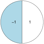
In each bet there is a certain chance to win and a certain chance to loss. The chances appear as an area the bets take in the pie. For example, in a bet,
there is a chance of fifty percent to win 1 NIS and a chance of fifty percent to lose 1 NIS and in a bet,
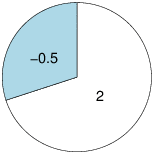
there is a chance of seventy percent to win 2 NIS and a chance of thirty percent to lose 0.5 NIS.
Participants’ mission was to choose between two bets. At the end of the experiment, one of the bets each participant marked was chosen. By means of a lottery (similar to roulette), a random place in the pie was chosen. According to this, it was determined whether the participant won or lost.
Table 1a: Payoff distribution of the 40 description-based prospects.
Win/loss amounts and probabilities in prospects: a, and b. Prospect b
is a more risky prospect in each a-b couple. R proportion is mean the
risky choice proportion (standard deviation in parenthesis).
Win a | Win | Loss a | Loss | Expected | Win b | Win | Loss b | Loss | Expected | R proportion |
prob. a | prob. a | value a | prob. b | prob. b | value b | |||||
| Low payoff | 0.56 (0.35) | |||||||||
1.54 | 87% | −3.46 | 13% | 0.89 | 1.92 | 77% | −3.08 | 23% | 0.77 | 0.60 (0.49) |
1.92 | 97% | −3.08 | 3% | 1.77 | 2.12 | 91% | −2.88 | 9% | 1.67 | 0.67 (0.47) |
4.32 | 3% | −0.68 | 97% | −0.53 | 2.33 | 88% | −2.67 | 12% | 1.73 | 0.81 (0.39) |
0.69 | 78% | −4.31 | 22% | −0.41 | 2.28 | 59% | −2.72 | 41% | 0.23 | 0.91 (0.29) |
4.44 | 31% | −0.56 | 69% | 0.99 | 0.40 | 63% | −4.60 | 37% | −1.45 | 0.17 (0.38) |
4.82 | 23% | −0.18 | 77% | 0.97 | 3.48 | 61% | −1.52 | 39% | 1.53 | 0.63 (0.49) |
1.98 | 11% | −3.02 | 89% | −2.47 | 0.14 | 82% | −4.86 | 18% | −0.76 | 0.75 (0.44) |
0.47 | 92% | −4.53 | 8% | 0.07 | 1.33 | 19% | −3.67 | 81% | −2.72 | 0.17 (0.38) |
4.44 | 38% | −0.56 | 62% | 1.34 | 3.17 | 89% | −1.83 | 11% | 2.62 | 0.31 (0.46) |
2.78 | 70% | −2.22 | 30% | 1.28 | 4.13 | 65% | −0.87 | 35% | 2.38 | 0.93 (0.25) |
1.45 | 5% | −3.55 | 95% | −3.30 | 0.27 | 38% | −4.73 | 62% | −2.83 | 0.60 (0.49) |
0.42 | 59% | −4.58 | 41% | −1.63 | 2.19 | 46% | −2.81 | 54% | −0.51 | 0.95 (0.23) |
4.10 | 30% | −0.90 | 70% | 0.60 | 2.32 | 67% | −2.68 | 33% | 0.67 | 0.45 (0.50) |
2.86 | 46% | −2.14 | 54% | 0.16 | 0.52 | 51% | −4.48 | 49% | −1.93 | 0.04 (0.20) |
4.80 | 16% | −0.20 | 84% | 0.60 | 4.67 | 65% | −0.33 | 35% | 2.92 | 0.99 (0.12) |
4.52 | 89% | −0.48 | 11% | 3.97 | 4.79 | 72% | −0.21 | 28% | 3.39 | 0.25 (0.44) |
1.67 | 99% | −3.33 | 1% | 1.62 | 1.92 | 51% | −3.08 | 49% | −0.53 | 0.04 (0.20) |
4.49 | 94% | −0.51 | 6% | 4.19 | 4.90 | 49% | −0.10 | 51% | 2.35 | 0.05 (0.23) |
1.05 | 69% | −3.95 | 31% | −0.50 | 4.29 | 35% | −0.71 | 65% | 1.04 | 0.87 (0.34) |
3.55 | 15% | −1.45 | 85% | −0.70 | 3.29 | 78% | −1.71 | 22% | 2.19 | 0.99 (0.12) |
| High payoff | 0.54 (0.34) | |||||||||
36 | 15% | −14 | 85% | −6.50 | 33 | 78% | −17 | 22% | 22.00 | 0.97 (0.16) |
10 | 69% | −40 | 31% | −5.50 | 43 | 35% | −7 | 65% | 10.50 | 0.83 (0.38) |
45 | 94% | −5 | 6% | 42.00 | 49 | 49% | −1 | 51% | 23.50 | 0.19 (0.39) |
15 | 5% | −35 | 95% | −32.50 | 3 | 38% | −47 | 62% | −28.00 | 0.65 (0.48) |
43 | 3% | −7 | 97% | −5.50 | 23 | 88% | −27 | 12% | 17.00 | 0.89 (0.31) |
19 | 97% | −31 | 3% | 17.50 | 21 | 91% | −29 | 9% | 16.50 | 0.37 (0.49) |
4 | 59% | −46 | 41% | −16.50 | 22 | 46% | −28 | 54% | −5.00 | 0.92 (0.27) |
15 | 87% | −35 | 13% | 8.50 | 19 | 77% | −31 | 23% | 7.50 | 0.64 (0.48) |
41 | 30% | −9 | 70% | 6.00 | 23 | 67% | −27 | 33% | 6.50 | 0.40 (0.49) |
44 | 31% | −6 | 69% | 9.50 | 4 | 63% | −46 | 37% | −14.50 | 0.11 (0.31) |
48 | 23% | −2 | 77% | 9.50 | 35 | 61% | −15 | 39% | 15.50 | 0.33 (0.47) |
17 | 99% | −33 | 1% | 16.50 | 19 | 51% | −31 | 49% | −5.50 | 0.04 (0.20) |
28 | 70% | −22 | 30% | 13.00 | 41 | 65% | −9 | 35% | 23.50 | 1.00 (0.00) |
20 | 11% | −30 | 89% | −24.50 | 1 | 82% | −49 | 18% | −8.00 | 0.73 (0.45) |
45 | 89% | −5 | 11% | 39.50 | 48 | 72% | −2 | 28% | 34.00 | 0.39 (0.49) |
32 | 89% | −18 | 11% | 26.50 | 44 | 38% | −6 | 62% | 13.00 | 0.32 (0.47) |
48 | 16% | −2 | 84% | 6.00 | 47 | 65% | −3 | 35% | 29.50 | 0.97 (0.16) |
5 | 92% | −45 | 8% | 1.00 | 13 | 19% | −37 | 81% | −27.50 | 0.09 (0.29) |
7 | 78% | −43 | 22% | −4.00 | 23 | 59% | −27 | 41% | 2.50 | 0.87 (0.34) |
29 | 46% | −21 | 54% | 2.00 | 5 | 51% | −45 | 49% | −19.50 | 0.01 (0.12) |
Table 1b: Payoff distributions of the ten experience-based tasks.
Each task consists of two buttons: a, and b. Button b is a more risky
button in each a-b couple. R represents the mean risky choice
proportion, wimth standard deviation in parenthesis.
| Task | Win a | Win | Loss a | Loss | Expected | Win b | Win | Loss b | Loss | Expected | R proportion | |
| prob. a | prob. a | Value a | prob. b | prob. b | Value b | |||||||
| 1 | 41 | 30% | −9 | 70% | 6.00 | 23 | 67% | −27 | 33% | 6.50 | 0.45 (0.26) | |
| 2 | 44 | 31% | −6 | 69% | 9.50 | 4 | 63% | −46 | 37% | −14.50 | 0.22 (0.16) | |
| 3 | 15 | 5% | −35 | 95% | −32.50 | 3 | 38% | −47 | 62% | −28.00 | 0.44 (0.17) | |
| 4 | 43 | 3% | −7 | 97% | −5.50 | 23 | 88% | −27 | 12% | 17.00 | 0.83 (0.11) | |
| 5 | 17 | 99% | −33 | 1% | 16.50 | 19 | 51% | −31 | 49% | −5.50 | 0.12 (0.13) | |
| 6 | 10 | 69% | −40 | 31% | −5.50 | 43 | 35% | −7 | 65% | 10.50 | 0.85 (0.14) | |
| 7 | 32 | 89% | −18 | 11% | 26.50 | 44 | 38% | −6 | 62% | 13.00 | 0.45 (0.30) | |
| 8 | 45 | 94% | −5 | 6% | 42.00 | 49 | 49% | −1 | 51% | 23.50 | 0.24 (0.25) | |
| 9 | 5 | 92% | −45 | 8% | 1.00 | 13 | 19% | −37 | 81% | −27.50 | 0.18 (0.16) | |
| 10 | 48 | 23% | −2 | 77% | 9.50 | 35 | 61% | −15 | 39% | 15.50 | 0.36 (0.21) | |
| Tasks average | 0.41 (0.19) | |||||||||||
Table 2a: Means and standard deviations (in parenthesis) of the BIC
scores and of the estimated model parameters in the two conditions of
the description-based tasks.
| Task | Model | BIC | Loss weight | Consistency | Sensitivity | Probability
discounting | Loss aversion |
| ProspectsH | PT | 14.90 (6.01) | NA | 3.42 (3.39) | 0.45 (0.35) | 0.34 (0.28) | 3.00 (3.23) |
PT-NO-S | 12.87 (6.69) | 0.56 (0.29) | 0.66 (1.27) | NA | 0.70 (0.28) | NA | |
Equality test stat. (2-tailed p-value) | 1.955 (0.0524) | ||||||
| ProspectsL | PT | 14.13 (5.98) | NA | 3.69 (3.01) | 0.58 (0.39) | 0.47 (0.36) | 1.41 (1.43) |
PT-NO-S | 12.80 (6.99) | 0.40 (0.24) | 1.65 (1.26) | NA | 0.74 (0.28) | NA | |
Equality test stat. (2-tailed p-value) | 1.252 (0.2126) | ||||||
| Note. Equality tests (t-statistics) refer to the hypothesis that the BIC scores of PT model are greater than those of PT-NO-S model. | |||||||
Table 2b: Means and standard deviations (in parenthesis) of the BIC scores and of the estimated model parameters across the 10 conditions of the experience-based tasks.
Task Model BIC Recency Loss weight Consistency Sensitivity Tasks Average EVL 7.26 (10.57) 0.34 (0.37) 0.52 (0.39) 2.93 (3.27) NA EVL-S 6.88 (10.65) 0.31 (0.37) 0.57 (0.38) 3.99 (3.73) 0.61 (0.40) Equality test stat. (2-tailed p-value) 0.219 (0.8266) EVL-PT 3.73 (7.60) 0.60 (0.42) NA 0.52 (1.20) 0.61 (0.38) Equality test stat. (2-tailed p-value) 2.349 (0.0204) Note. Equality tests (t-statistics) refer to the hypothesis that the BIC score of the EVL model is equal to that of the EVL-S model and EVS-PT model, separately.
Table 3a: Average G 2 scores, standard deviations (in parenthesis), and percent of individuals for which the generalization prediction is better than a random model (success proportion) in description-based tasks.
PT Source condition Average G2 score Success proportion ProspectsL −9.85 (24.02) 0.48 ProspectsH −1.54 (16.95) 0.63 Prospects Average −5.69 (20.48) 0.55 PT-NO-S Source condition Average G2 score Success proportion ProspectsL −18.54 (26.51) 0.33 ProspectsH −3.70 (6.29) 0.93 Prospects Average −7.42 (16.40) 0.63
Table 3b: AverageG 2 scores, standard deviations (in parenthesis), and percent of individuals for which the generalization prediction is better than a random model (success proportion) in experience-based tasks, averaged across the 10 conditions.
EVL Average G2 score Success proportion −43.57 (116.68) 0.51 EVL-S Average Success proportion −65.40 (137.40) 0.44 EVL-PT Average Success proportion −63.58 (104.51) 0.46
Table 4a: Two-sided Spearman correlations between parameter values estimated in the description-based high and low-payoff tasks.
Model Loss weight Consistency Sensitivity Probability discounting Loss aversion PT NA 0.09 0.22 0.23* 0.20 PT-NO-S 0.33* 0.40* NA 0.56* NA Note. Asterisks denote significance at 5% level (two-tailed p-values).
Table 4b: Average two-sided Spearman correlations between parameter values estimated in the experience-based tasks.
Model Recency Loss weight Consistency Sensitivity EVL 0.081 (0.114)* 0.080 (0.134)* 0.092 (0.103)* NA EVL-S 0.010 (0.190) 0.060 (0.230)* −0.060 (0.410)* −0.12 (0.60)* EVL-PT −0.048 (0.200)* NA −0.029 (0.488) −0.03 (0.28) Note. Standard deviations of the correlations are shown in parentheses. Asterisks denote significance at 5% level (two-tailed p-values).
Table 5: Two-sided Spearman correlations between the values of the same or similar parameters estimated in the description-based and the experience-based tasks.
Experience − Description model Loss weight Consistency EVL − PT-NO-S 0.12 −0.12 EVL-S − PT-NO-S 0.22* −0.10 EVL − PT 0.03 0.07 EVL-S − PT −0.23 0.02 Asterisks denote significance at 5% level (two-tailed p-values).
| V(xai)= |
|
| θ=(t/10)c |
| u(t)=win(t)a−β · loss(t)a |
This document was translated from LATEX by HEVEA.