Judgment and Decision Making, vol. 6, no. 6, August 2011, pp.
439-519
Using the ACT-R architecture to specify 39 quantitative process models of decision makingJulian N. Marewski* Katja
Mehlhorn# |
Hypotheses about decision processes are often formulated qualitatively
and remain silent about the interplay of decision, memorial, and other
cognitive processes. At the same time, existing decision models are
specified at varying levels of detail, making it difficult to compare
them. We provide a methodological primer on how detailed cognitive
architectures such as ACT-R allow remedying these problems. To make our
point, we address a controversy, namely, whether noncompensatory or
compensatory processes better describe how people make decisions from
the accessibility of memories. We specify 39 models of
accessibility-based decision processes in ACT-R, including the
noncompensatory recognition heuristic and various other popular
noncompensatory and compensatory decision models. Additionally, to
illustrate how such models can be tested, we conduct a model
comparison, fitting the models to one experiment and letting them
generalize to another. Behavioral data are best accounted for by race
models. These race models embody the noncompensatory recognition
heuristic and compensatory models as a race between competing
processes, dissolving the dichotomy between existing decision models.
Keywords: ACT-R, noncompensatory and compensatory models, recognition
heuristic, race models, cognitive architectures.
1 Introduction
Even if the mind has parts, modules, components, or whatever, they all
mesh together to produce behavior. ... If a theory covers only one part
or component, it flirts with trouble from the start. (A. Newell, 1990,
p. 17)
One way to increase the precision of theories of decision making is to
specify the cognitive processes decision-making mechanisms are assumed
to draw on. Corresponding process models predict not only
what decision a person will make, but also how the information used to
make the decision will be processed. The past decades have seen
repeated calls to develop process models, and in fact, such models
have become increasingly popular (e.g., Brandstätter, Gigerenzer, &
Hertwig, 2006; Einhorn, Kleinmutz, & Kleinmutz, 1979; Ford, Schmitt,
Schechtman, Hults, & Doherty, 1989; Gigerenzer & Goldstein, 1996;
Gigerenzer, Hoffrage, & Kleinbölting, 1991; Marewski, Gaissmaier,
Gigerenzer, 2010a, 2010b; Payne, Bettman, & Johnson, 1988, 1993;
Schulte-Mecklenbeck, Kühberger, & Ranyard, 2010). The predictions
made by these models have motivated a number of debates; for example,
whether people rely on noncompensatory, lexicographic as opposed to
compensatory, weighted-additive processes in inference, choice, and
estimation (e.g., Bergert & Nosofsky, 2007; Bröder & Schiffer,
2003, 2006; Cokely & Kelley, 2009; von Helversen & Rieskamp, 2008;
Johnson, Schulte-Mecklenbeck, & Willemsen, 2008; Lee & Cummins,
2004; Marewski, 2010; Mata, Schooler, & Rieskamp, 2007; B.R. Newell,
Weston, & Shanks, 2003; Nosofsky & Bergert, 2007; Rieskamp &
Hoffrage, 1999, 2008; Rieskamp & Otto, 2006).
Yet, often such process models are underspecified relative to the
process data against which they can be tested. In this article, we show
how precision can be lent to process models by implementing them in a
cognitive architecture. We will make our point by focusing on a class
of models that assume people to make decisions by exploiting the
accessibility (e.g., Bruner, 1957; Higgins, 1996; Kahneman,
2003) of memory contents. These models have been at the focus of a
debate about what processes describe people’s decisions
best when they make inferences about unknown states of the world; such
as when predicting which sports teams are likely to win a competition,
which politician will win an election, or which cities are likely to
grow fastest in the number of inhabitants.
1.1 A case study of underspecified process hypotheses
Numerous accessibility-based decision models have been proposed,
featuring concepts such as familiarity, fluency, availability, or
recognition (e.g., Dougherty, Gettys, & Ogden, 1999; Jacoby & Dallas,
1981; Koriat, 1993; Pleskac, 2007; Tversky & Kahneman, 1973). One such
model is the recognition heuristic (Goldstein & Gigerenzer,
2002). As suggested by its name, this simple decision strategy operates
on our ability to discriminate between recognized alternatives
that we have encountered in our environment before, and
unrecognized ones that we do not remember to have seen or
heard of before. In doing so, the heuristic can help us to infer which
of two alternatives (e.g., two cities, York and Stockport), one
recognized and the other not, has the larger value on an unknown
criterion (e.g., city size). The heuristic reads as follows:
If only one of two alternatives is recognized, infer the
recognized one to be larger.
The recognition heuristic is a noncompensatory model for memory-based
decisions: Even if further knowledge beyond recognizing an alternative
is retrieved, this knowledge is ignored when the heuristic is used.
Instead, the decision is based solely on recognition. In contrast to
the recognition heuristic and related accessibility-based heuristics
(e.g., Schooler & Hertwig, 2005), many other decision models posit
that people evaluate alternatives by using knowledge about their
attributes as cues (Bröder & Schiffer, 2003, Hauser &
Wernerfelt, 1990; Lee & Cummins, 2004; Payne et al., 1993). For
instance, to infer which of two cities is larger, a person could rely
on one of the classic compensatory unit-weight linear
integration strategies (e.g., Dawes, 1979): The person could
recall whether the cities have industry sites, airports, or famous
soccer teams. For each city, the person could count the number of
positive and negative cues (e.g., having an airport
would be a positive cue and lacking one a negative cue) and then infer
the city with the larger sum to be larger (Einhorn & Hogarth,
1975; Gigerenzer & Goldstein, 1996; Huber, 1989). The assumption in
such compensatory models is that an alternative’s value
on one cue is traded off against its value on another cue.
1.2 Process hypotheses in the memory paradigm
The recognition heuristic has triggered a debate about what processes
describe people’s decisions best when they make inferences from the
accessibility of memories: Do people rely on this noncompensatory
heuristic, ignoring further knowledge, or do they use compensatory
strategies instead? (Bröder & Eichler, 2006; Davis-Stober, Dana, &
Budescu, 2010; Dougherty, Franco-Watkins, & Thomas, 2008; Erdfelder,
Küpper-Tetzel, & Mattern, 2011; Gaissmaier & Marewski, 2011;
Gigerenzer & Brighton, 2009; Gigerenzer & Goldstein, 2011;
Gigerenzer, Hoffrage, & Goldstein, 2008; Glöckner & Bröder,
2011; Goldstein & Gigerenzer, 2011; Hertwig, Herzog, Schooler, &
Reimer, 2008; Hilbig, Erdfelder, & Pohl, 2010; Hilbig & Pohl, 2009;
Hochman, Ayal, & Glöckner, in 2010; Hoffrage, 2011; Marewski,
Gaissmaier, Schooler, Goldstein, & Gigerenzer, 2009, 2010; Marewski,
Pohl, & Vitouch, 2010, 2011a, 2011b; McCloy, Beaman, & Smith, 2008;
B. R. Newell & Fernandez, 2006; B. R. Newell & Shanks, 2004;
Oeusoonthornwattana & Shanks, 2010; Oppenheimer, 2003; Pachur, 2010,
2011; Pachur & Biele, 2007; Pachur & Hertwig, 2006; Pachur, Mata, &
Schooler, 2009; Pachur, Todd, Gigerenzer, Schooler, & Goldstein,
2011; Pohl, 2006; 2011; Reimer & Katsikopoulos, 2004; Richter &
Späth, 2006; Scheibehenne & Bröder, 2007; Volz et al., 2006).
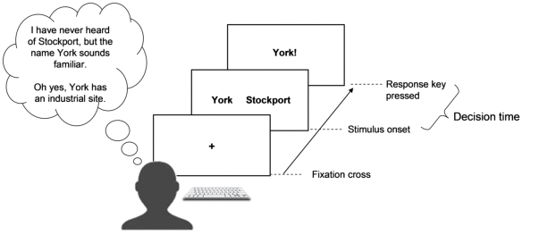
In this debate, many researchers have used the memory paradigm
shown in Figure 1. The time it takes a person to make the
decision—the decision time measured from stimulus onset
until the person presses a key—is used to test hypotheses about the
processes underlying the decision (e.g., Hertwig et al., 2008; Hilbig
& Pohl, 2009; Marewski, Gaissmaier, Schooler, et al., 2010; Richter &
Späth, 2006; Volz et al., 2006). For instance, Pachur and Hertwig
(2006) hypothesized that recognition memory would be more easily
assessed than memories about cues, enabling people to make decisions
based on the recognition heuristic faster than decisions based on cues.
| Figure 1: The memory paradigm. In a two-alternative
forced-choice task, on a computer screen a person is first shown a
fixation cross, and thereafter presented with the names of two
alternatives (e.g., two city names). The person’s task
is to infer which of the two has a larger value on the criterion (e.g.,
which of two cities is larger). To make this decision, the person has
to retrieve all information she wants to use from memory. For instance,
the person may believe to recognize a city’s name and
additionally remember that the city has an industrial site, suggesting
that it is a large city. Once a person has made her decision, she
presses a key to respond. Gigerenzer and Goldstein (1996) referred to
such experimental paradigms as inferences from memory. |

Importantly, although tests of such process hypotheses are central to
the debate about the recognition heuristic, thus far the hypotheses put
forward in this debate lack precision. First, in the memory paradigm,
in no study were decision times actually quantitatively predicted.
Rather, mostly qualitative (e.g., ordinal) decision time hypotheses were
tested. Second, in no study these hypotheses took into account the
interplay among perceptual, memory, decision, intentional, and motor
processes governing decision times in the memory paradigm (but see
Marewski, 2008; Marewski & Schooler, 2011). In a recent test of
process hypotheses with the memory paradigm, Hilbig and Pohl (2009),
for example, derived qualitative decision time hypotheses for the
recognition heuristic and compared them against corresponding
hypotheses they derived from evidence accumulation processes,
as they have been outlined by B. R. Newell (2005) and others (e.g., Lee
& Cummins, 2004). Broadly speaking, the assumption of such evidence
accumulation processes is that evidence (e.g., cues and other
information) for each of two alternatives is accumulated sequentially
until a decision threshold is reached (e.g., C cues are
retrieved) and a decision made (e.g., in favor of the alternative with
most accumulated evidence). In testing their hypotheses, Hilbig and
Pohl subsumed a number of models under this broad notion of evidence
accumulation, including a connectionist parallel constraint
satisfaction model (Glöckner & Betsch, 2008), and decision
field theory (Busemeyer & Townsend, 1993). According to them, their
decision time data could be accounted for by compensatory evidence
accumulation models but were inconsistent with the recognition
heuristic. However, Hilbig and Pohl did not actually specify a single
evidence accumulation model, and correspondingly, they also did not
apply any model to their data. This is problematic, as different
evidence accumulation models will make different predictions, depending
on the specific model and its parameter values. Moreover, the
recognition heuristic on its own does not make predictions about
decision times in the memory paradigm (see also Gigerenzer &
Goldstein, 2011, for a discussion).
In the memory paradigm, decision times are subject, at least, to the
following: the time it takes to read alternatives’ names, the time it
takes to judge alternatives as recognized or unrecognized, the time it
takes to retrieve cues about the alternatives, the time it takes to
make a decision as to which alternative to pick, and the time it takes
to press a key. In addition a person’s intentions (e.g., to respond as
quickly as possible) can affect decision times. As a result, decision
time predictions warrant not only a model of decision making, but also
models of how decision processes interplay with other processes. The
recognition heuristic, as formulated by Goldstein and Gigerenzer
(2002), remains silent about this interplay; and so do, in fact, most
other accessibility-based models of decision making that have been
tested in the memory paradigm, including the evidence accumulation and
parallel constraint satisfaction models Hilbig and Pohl (2009) focused
on.1
1.3 Overview
In this article, we will model the respective contributions of
perceptual, memory, decision, intentional, and motor processes by
quantitatively specifying a number of the process hypotheses that have
been formulated in the literature in a cognitive architecture.
A cognitive architecture is a quantitative theory that applies to a
broad array of behaviors and tasks, formally integrating theories of
memory, perception, action, and other aspects of cognition (for an
introduction to cognitive architectures, see e.g., Gluck, 2010). Among
the architectures developed to date (e.g., EPIC, Meyer &
Kieras, 1997; Soar, A. Newell, 1992), the ACT-R
architecture (e.g., Anderson, et al., 2004) provides perhaps
the most detailed account of the various processes that may play a role
in accessibility-based decisions. ACT-R has been successfully used to
explain phenomena in a variety of fields, ranging from list memory
(Anderson, Bothell, Lebiere, & Matessa, 1998), visuospatial working
memory (e.g., Lyon, Gunzelmann, & Gluck, 2008), diagnostic reasoning
(Mehlhorn, Taatgen, Lebiere, & Krems, in press), and probability
learning (Gaissmaier, Schooler, & Rieskamp, 2006) to flying (Gluck,
Ball, & Krusmark, 2007), driving (Salvucci, 2006), and the teaching of
thousands of children in U.S. high schools with tutoring systems
(Ritter, Anderson, Koedinger, & Corbett, 2007). Here, we will use
ACT-R to implement 39 process models. These models are the recognition
heuristic, as well as various other noncompensatory and compensatory
decision strategies, including models that incorporate central aspects
of integration, connectionist, evidence accumulation, and race models.
In a model competition, we will test the 39 process
models’ ability to predict people’s
decisions and decision times in the memory paradigm.
Before we start, three comments are warranted. First, the goal of this
article is not so much to advocate any particular process model, but
rather, using the debate about the recognition heuristic as a case
study, to provide a methodological primer on how architectures like
ACT-R can be used to lend precision to the theorizing about decision
processes. That is, while we also test process models against each
other, the model competition’s objective is to illustrative
methodological principles, and not necessarily to identify the very
best model. For those interested in identifying the best model, the
main contribution of this article is, perhaps, to provide 39 precisely
specified process models, cast into the computer code of a detailed
cognitive architecture, and ready to be tested in studies beyond the
limited data we use here.
Second, there are many research programs that are built around
quantitative models (e.g., Busemeyer & Townsend, 1993; Ratcliff &
Smith, 2004; Rumelhart, McClelland, & the PDP Research Group, 1986).
Certainly, our critique of the lack of specification of process
hypotheses only applies to these models to the extent that they remain
silent about the interplay of perceptual, memory, decision,
intentional, and motor processes. Moreover, we are not the first who
discuss decision strategies such as the recognition heuristic and
related models in the context of ACT-R or other architectures (e.g.,
Dougherty et al., 2008; Gaissmaier, Schooler, & Mata, 2008; Hertwig et
al., 2008; Marewski & Schooler, 2011; Nellen, 2003; Schooler &
Hertwig, 2005; Van Maanen & Marewski, 2009).
Third, while it is possible to test evidence accumulation, the
recognition heuristic, and other models against each other without
implementing these models in a cognitive architecture, such
direct model comparisons are not without problems, because
these models tend to be specified at different levels of description
and computational precision, resulting in different levels of detail
and precision of the models’ predictions. For instance,
many evidence accumulation models are specified mathematically and
include several free parameters (e.g., Ratcliff & Smith, 2004). The
recognition heuristic, in turn, consists of a verbally formulated
if-then statement. (If one alternative is recognized, then choose the
recognized alternative.) While the parameterized evidence accumulation
models can yield predictions about decision time distributions, on its
own the recognition heuristic’s if-then-statement does
not predict such distributions. Much the same can be said with respect
to comparisons of other models, including the aforementioned parallel
constraint satisfaction and classic integration models. By implementing
models of different levels of description and specificity in
one architectural modeling framework, we make the models and
their predictions comparable, providing a basis for future model tests
beyond the ones we will provide below.
The article is structured as follows. First, we will describe the
experimental data we used to test the models. Second, we will explain
the methodological principles guiding our modeling. Third, we will
provide an overview of ACT-R as well as of the models we implement.
Fourth, we will illustrate how these models’ ability to
predict people’s decisions and decision times can be
tested.
2 Experimental data
We developed models for memory-based decisions about city size, which
is the task most studies on the recognition heuristic have used
(Figure 1). Specifically, we reanalyze Pachur, Bröder, and
Marewski’s (2008) Experiments 1 and 2.2 These experiments are well-suited for our purposes,
because they entail good control over peoples’ recognition and
cue-knowledge, this way simplifying our modelling exercise.
2.1 Summary of Pachur et al.’s (2008) pre-studies
To create stimulus materials for their experiments, Pachur et al. (2008)
conducted pre-studies wherein they presented participants with names of
British cities and had them indicate whether they had heard or seen the
names prior to participating in the study, that is, whether they
recognized them. Six highly recognized and 10 poorly recognized cities
(R cities and U cities, respectively) were selected
as stimuli. Pachur et al. also surveyed what people thought were useful
cues for inferring the cities’ sizes to establish a
stimulus set of cues. These cues were whether a city had significant
industry (industry cue), an international airport
(airport cue), or a premier league soccer team (soccer
cue).
2.2 Summary of Pachur et al.’s (2008) Experiment 1
Learning task. The experiment was run with a new group
of participants (N = 40, 19 females; mean age = 24.6 years).
The experiment started with a learning task (as used by Bröder &
Eichler, 2006; Bröder & Schiffer, 2003), in which participants were
taught the three cues about the six R cities. During learning, cities
and cues were presented repeatedly in a random order until participants
correctly recalled all cities’ values on the cues.
Table 1 summarizes the cues.
| Table 1: Cues taught in the learning tasks of Experiments 1 and 2. |
| | City |
|
Cue | Aberdeen | Bristol | Nottingham | Sheffield | Brighton | York |
| Industry | + | + | + | + | +/−a | +/−a |
| Airport | + | + | − | − | − | − |
| Soccer | + | + | + | + | − | − |
| Note. + = positive cue value. − = negative cue value. |
| a The design of Experiment 1 and 2 differed slightly.
In Experiment 1, Pachur et al. (2008) taught participants positive
values on the industry cue for Brighton and York. In Experiment 2,
Pachur et al. taught participants negative values on the industry cue
for Brighton and York. |
Decision task. After having learned the cues, participants
performed the decision task. In this task, 120 pairs of
British cities were presented on a computer screen (one city on the
left side of the screen, the other on the right). Participants were
instructed to choose the one with more inhabitants by pressing a key
(Figure 1).
For each trial, a pair of cities was drawn at random from
three types of city pairs. In the main type (i), six R cities that
were mostly recognized in the pre-studies were combined with 10 cities
that were mostly unrecognized in the pre-studies, yielding 60
RU pairs. These 60 pairs were critical for Pachur et al.’s
(2008) and our purposes, because they were most likely to allow people
to apply the recognition heuristic. We used these pairs to test our
models. To balance the presentation frequency of the R and U cities as
much as possible, (ii) there were 30 filler pairs consisting of two
cities that were mostly unrecognized in the pre-studies (UU
pairs) as well as (iii) 30 filler pairs consisting of two
recognized cities (RR pairs).
Recognition task. The decision task was followed by a
recognition task. Participants were presented all cities in a
random order and had to indicate for each city whether they had heard
of it before participating in the experiment. The purpose of this
recognition task was to make sure that the RU pairs, which were
identified based on the pre-studies, also represented RU pairs for the
participants of Experiment 1, whose recognition judgments were likely
to be similar but not identical to the recognition judgments made in
the pre-studies. We used participants’ responses in
this task to model their recognition of cities.
Cue-memory task. After the recognition task, participants
performed a cue-memory task in which they had to reproduce
the cue values (“yes” or “no”) they had learned for the six R
cities in the learning task. If they could not recall the correct
values, they were allowed to respond “don’t know”. The purpose of
this task was to test how well participants remembered the cues they
were taught. We used participants’ responses in this task to model
their retrieval of cues; for instance, whether they believed a city to
have an airport.
2.3 Summary of Pachur et al.’s (2008) Experiment 2
In Experiment 2 (N = 40; 25 females; mean age = 25.2 years),
for two cities the positive values on the industry cue were replaced by
negative ones, such that recognition was contradicted by three negative
cues (Table 1). In all other respects, Experiment 2 was identical to
Experiment 1.
3 Model-testing approach: Methodological principles
To strengthen our modeling efforts, we embraced five methodological
principles.
Nested modeling. Any new model should be related to its own
precursor (e.g., including it as special cases) and should be tested on
data that the old model was able to account for (Grainger & Jacobs,
1996; Jacobs & Grainger, 1994). Our models implement the qualitative
hypotheses discussed in the literature in a stepwise, nested fashion,
and are tested on Pachur et al.’s (2008) data.
Competitive modeling. A model’s ability to
account for data should not be evaluated in isolation, but in model
comparisons (e.g., Fum, Del Missier, & Stocco, 2007; Gigerenzer &
Brighton, 2009; Marewski, Schooler, & Gigerenzer, 2010). In such
comparisons, a model’s ability to account for data can
be compared to that of competing models. For instance, this way it is
possible to learn that no model accounts for the data perfectly, but some
account for them better than others. This way it is also possible to
establish benchmarks in model evaluation; for example, a new model
should be able to account for data better than previously existing
models that are already known to account well for that data.
Unfortunately, this competitive approach to model testing has rarely
been taken in recognition heuristic research (but see Glöckner &
Bröder, 2011; Marewski, Gaissmaier, Schooler, et al., 2009, 2010,
Pachur & Biele, 2007, for exceptions). Here, we test all models
competitively.
| Figure 2: The organization of ACT-R. Note that the
modules of the architecture have been mapped onto brain regions,
enabling detailed process predictions of functional magnetic resonance
imaging (fMRI) data (see e.g., Anderson, Fincham, Qin, & Stocco,
2008). While it is beyond the scope of this article to test fMRI
predictions, we would like to point out that all models reported in
this article actually allow making such predictions, inviting future
model tests. |

Constrained modeling. Models should be tested by constraining
their parameters in separate tasks (Anderson, 2007; Newell, 1990). We
calibrated all models’ free parameters to the tasks of
Experiment 1, using a stepwise procedure to constrain the parameter
space. Specifically, we first fitted the parameters associated
with recognition and cue retrieval on data of the recognition and
cue-memory tasks of Experiment 1, creating separate ACT-R models of
recognition and cue retrieval. With these parameters fixed, we
then estimated the remaining parameters from
participants’ decisions and decision times in the
decision task of Experiment 1 (Appendix A).
Predictive modeling. We use the term “predicting” (or
“generalization”) to refer to
situations in which a model’s free parameters are fixed such that
they cannot adjust to the data on which the model is tested. In
contrast, we reserve the term “fitting” (or “calibration”) to
refer to situations in which a model’s parameters are allowed to
adapt to the data. Predicting data well lends credence to a model
and is one standard by which models should be evaluated (e.g.,
Busemeyer & Y. M. Wang, 2000; Marewski & Olsson, 2009; Pitt, Myung,
& S. Zhang, 2002; Roberts & Pashler, 2000). We used the parameters
fitted on Experiment 1 to predict behavior in Experiment 2.3
Distributional modeling. Rather than just predicting means of
behavioral data, we strive to predict the associated distributions,
which further helps evaluating our ACT-R models’ ability to account
for human data (for a related approach, see Ratcliff & Smith,
2004). Next, we will turn to ACT-R and these models.
4 Thirty-nine ACT-R models of inference
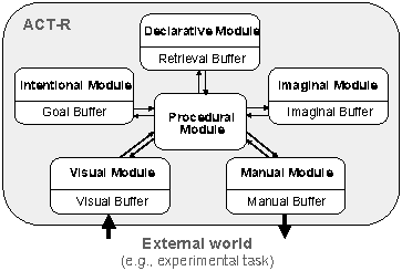
ACT-R describes human cognition as a set of independent modules that
interact through a production system (Figure 2). The production system
consists of production rules (i.e., if–then rules) whose
conditions (i.e., the “if” parts of the rules) are matched against
the modules. If the conditions of a production rule are met, then the
production rule can fire. In this case, the action specified by the
production rule is carried out.
Each module implements different cognitive processes. The
declarative module allows information storage in and retrieval
from declarative memory, the intentional module keeps track of
a person’s goals, and the imaginal module
holds information necessary to perform the current task. By this token,
the imaginal module is comparable to the focus of attention in working
memory (e.g., Anderson, 2007; Borst, Taatgen, & Van Rijn, 2010;
Oberauer, 2002). A visual module for perception and a
manual module for motor actions (e.g., pressing a key on a
computer keyboard) are used to simulate interactions with the world.
While the different modules can operate in parallel, information within
each module can only be processed in a serial manner (Byrne &
Anderson, 2001).
In coordinating the modules, the production rules can act only on
information that is available in buffers, which can be thought
of as processing bottlenecks (Salvucci & Taatgen, 2008), linking the
modules’ contents to the production rules. For
instance, the production rules cannot access all contents of the
declarative module, but only the part of information that is currently
available in the retrieval buffer.
ACT-R distinguishes a symbolic and a
subsymbolic system. The symbolic system is composed
of the production rules as well as the modules and buffers. Access to
the information stored in the modules and buffers is determined by the
subsymbolic system. This system is cast as a set of equations and
determines, for instance, the timing of memory retrieval. Before
turning to these equations, let us provide two examples of the ACT-R
models we implemented.
4.1 Implementing accessibility-based decision strategies in
ACT-R: Two examples
Our ACT-R models perform the same decision task as Pachur et al.’s
experimental participants: They “read” the city names off the
computer screen, process them, decide which city is larger, and enter
the response by “pressing” a key.
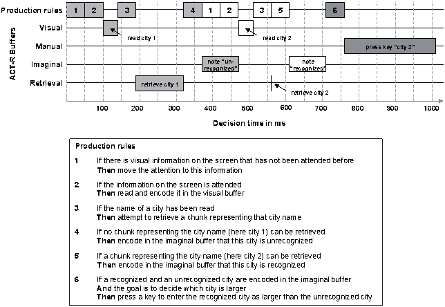
| Figure 3: Processing stream for Model 1, one of our
implementations of the recognition heuristic. Light grey boxes depict
processing an unrecognized city name; white boxes depict processing a
recognized city name. Dark grey boxes depict actions related to the
response. Note that predicted decision times represent examples; the
model’s decision time predictions can vary across
different decision trials, for instance, as a function of noisy
perceptual and motor processes (Appendix A). Production rules are
stylized representations of the LISP code productions rules that have
been used to implement the models in ACT-R. |

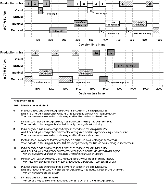
| Figure 4: Processing stream for Model 4.H.PN. Light
grey boxes depict processing an unrecognized city name; white boxes
depict processing a recognized city name. Striped boxes depict actions
related to the retrieval of cues. Dark grey boxes depict actions
related to the response. Note that predicted decision times represent
examples; the model’s decision time predictions can
vary across different decision trials, for instance, as a function of
noisy perceptual and noisy motor processes, or as a function of whether
to-be-retrieved cues are positive, negative, or unknown (Appendix A).
As we explain in detail below, also the order in which cues are
processed (i.e., productions 6–11) will vary across trials (see also
Footnote 7). Production rules are stylized representations of the LISP
code productions rules that have been used to implement the models in
ACT-R. |

Figure 3 shows the processing stream of Model 1, which is one of our
recognition heuristic implementations. As can be seen, the various
processing steps assumed by the model are coordinated by a set of
production rules. Specifically, the model assumes that people first
read the names of both cities. In doing so, the model attempts to
retrieve a memory trace of the cities’ names, called a
chunk. Chunks are facts like “York is a city” or “York has
industry” and model people’s recognition of city names and their cue
knowledge, respectively. If a chunk representing the name of one city
can be retrieved, then this city is recognized.4 In Model 1, retrieving the chunk of one city but
not the chunk of the other is sufficient information to enter the
recognized city as the larger city.
To compare, Figure 4 shows one of the compensatory strategies we
implemented. As can be seen, Model 4.H.PN assumes that, after assessing
recognition, a person will retrieve chunks about the recognized city,
such as the industry cue. The retrieved cues are stored in the imaginal
buffer. As we will explain below, from the imaginal buffer the cues
spread a memory signal called activation to intuitive
knowledge that large cities tend to have airports, premier league
soccer teams, and significant industry. In the model, this knowledge is
labeled big chunk. If the big chunk receives sufficient
spreading activation from the retrieved cues, then Model 4.H.PN will
recall that the recognized city is a large city and enter this city as
response. If the big chunk’s activation is too weak,
then the big chunk will not be retrieved. Consequently, the model has
no reason to assume that the recognized city is large and will respond
with the unrecognized city. The assumption is that such subsymbolic
processes describe how people make implicit and intuitive, rather than
explicit, deliberate judgments.
As can be seen by comparing the x-axes of Figures 3 and 4, decision
times are longer in Model 4.H.PN than in Model 1, because Model 4.H.PN
assumes more processing steps than Model 1. In what follows, we give a
short overview of the subsymbolic processes that determine the timing
of the processing steps in these and all other models.
4.2 Subsymbolic memory processes assumed by ACT-R
Access to chunks such as “York is a city” or “York has industry”
is determined by the chunk’s activation (Lovett, Daily, & Reder,
2000). The activation, Ai,
of chunk i (e.g., a city or a cue) reflects the likelihood
that the chunk will be needed in the future (Anderson & Schooler,
1991) and is determined by three components—the chunk’s
base-level activation, Bi,
the spreading activation the chunk receives from the current
context, Si, and a noise
component, ε:
The first component that influences a chunk’s
activation, Ai, its base-level
activation, Bi, reflects the
chunk’s past usefulness:
| Bi = ln | ⎛
⎜
⎜
⎝ | | tk−d
| ⎞
⎟
⎟
⎠ | (2) |
where n is the number of
presentations of chunk i,
tk is the time since the
kth presentation, and d
is a decay parameter. Consequently, the more often a city name or a
cue was encountered (e.g., in an experimental task) and the more
recent these encounters were, the higher the city’s or cue’s
activation.5
The second component that influences a chunk’s activation,
Ai, spreading activation,
Si, reflects the chunk’s usefulness
in the current context. The amount of spreading activation is
determined by the chunk’s association to other chunks that are
currently stored in the buffers (Anderson & Lebiere, 1998). In
our models, reading a city name and encoding it in the imaginal buffer
would, for example, increase the likelihood of a cue associated with
this city being needed. The city would spread activation to the cue as
described by Equation 3:
where cue i receives spreading activation,
Si, from city j. The amount
of spreading activation Si is
determined by the associative strength,
Sji, between i and
j, which is weighted by the source
activation, Wj, of
j in the imaginal buffer. The associative strengths,
Sji, between chunks is approximated
with
| Sji = S − ln (fanji), (4) |
where S is a parameter for the maximum associative
strength between chunks and fan is the number of chunks
i that are associated with a chunk j. Consequently,
the more cues are associated with a city in memory, the lower the
associative strength between the city and each of the cues.
The third component that influences a chunk’s
activation, Ai, is the retrieval
noise, ε . It is added to the activation of a
chunk when a retrieval request is made. With s being a free
parameter, ε is generated from a
logistic distribution with a mean of zero and a variance of
Only chunks that exceed a certain amount of activation,
Ai, as defined by the
retrieval threshold, τ , can be retrieved. For instance,
only cues with activations falling above τ would be retrieved.
The retrieval probability, p, is:
p = 1/{1 + e(τ - Ai)/s}
If a chunk i can be retrieved, the time required for the
retrieval is determined by the latency factor, F, and
the activation of the chunk, Ai:
| retrieval time = Fe−Ai. (6) |
Thus, the more strongly city names and cues are activated in memory the
faster they can be retrieved.
If no chunk matches a retrieval request or if the matching chunk with
the highest activation is below the retrieval threshold, a retrieval
failure will occur. For example, reading the name of an unknown city
will result in a retrieval failure. The time it takes to note such a
failure is:
| retrieval time = Fe−τ. (7) |
4.3 Detailed description of the 39 models
The above-described subsymbolic memory processes as well as the
corresponding parameter values are identical in all models and the
models also do not differ with respect to the perceptual and motor
processes they assume (Appendix A).
However, the models do differ with respect to the decision
processes. In implementing these processes, we had to make a series of
assumptions, for instance, about the order in which people will assess
recognition as opposed to cues. All assumptions are grounded in the
decision, memory, and ACT-R literatures. Often, however, these
literatures offer more than one plausible assumption. Following the
principle of competitive modeling, we dealt with such competing
assumptions by creating different models to implement them, which
allowed us to test the assumptions against each other. Following the
principle of nested modeling, we additionally combined part of these
assumptions with each other, resulting in 39 models. These models are
summarized in Table 2.
Table 2a: Overview of the perception and memory processes used in the
39 models.| | Retrieve and encode city names | Retrieve positive cues | Retrieve negative cues | Number of retrieved cuesa | Retrieved cues can be forgotten | Encode cues in the imaginal buffer |
| Model 1 class: Stopping and decision rules noncompensatory—simple model |
| Model 1 | X | | | 0 | | |
| Model 2 class: Stopping rule compensatory, decision rule noncompensatory—simple models |
| Model 2.PN | X | X | X | 3 | | |
| Model 2.P | X | X | | 3 | | |
| Model 3 class: Stopping rule compensatory, decision rule noncompensatory—simple models |
| Model 3.PN | X | X | X | 3 | | X |
| Model 3.P | X | X | | 3 | | X |
| Model 1&3 class: Stopping rule
noncompensatory and compensatory, decision rule noncompensatory—race models |
| Model 1&3.PN | X | X | X | 0 to 3 | | X |
| Model 1&3.P | X | X | | 0 to 3 | | X |
| Model 1&3.PN.F | X | X | X | 0 to zb | X | X |
| Model 1&3.P.F | X | X | | 0 to zb | X | X |
| Model 4 class: Stopping rule
compensatory, decision rule compensatory—simple
models |
| Model 4.H.PN | X | X | X | 3 | | X |
| Model 4.H.P | X | X | | 3 | | X |
| Model 4.L.PN | X | X | X | 3 | | X |
| Model 4.L.P | X | X | | 3 | | X |
| Model 1&4 class: Stopping
rule noncompensatory and compensatory, decision rule noncompensatory and
compensatory—race models |
| Model 1&4.H.PN | X | X | X | 0 to 3 | | X |
| Model 1&4.H.P | X | X | | 0 to 3 | | X |
| Model 1&4.H.PN.F | X | X | X | 0 to zb | X | X |
| Model 1&4.H.P.F | X | X | | 0 to zb | X | X |
| Model 1&4.L.PN | X | X | X | 0 to 3 | | X |
| Model 1&4.L.P | X | X | | 0 to 3 | | X |
| Model 1&4.L.PN.F | X | X | X | 0 to zb | X | X |
| Model 1&4.L.P.F | X | X | | 0 to zb | X | X |
| Model 5 class: Stopping rule
compensatory, decision rule compensatory—simple models |
| Model 5.1.PN | X | X | X | 1 to 3 | | X |
| Model 5.1.P | X | X | | 1 to 3 | | X |
| Model 5.2.PN | X | X | X | 2 to 3 | | X |
| Model 5.2.P | X | X | | 2 to 3 | | X |
| Model 5.3.PN | X | X | X | 3 | | X |
| Model 5.3.P | X | X | | 3 | | X |
| Model 1&5 class: Stopping
rule noncompensatory and compensatory, decision rule noncompensatory and
compensatory—race models |
| Model 1&5.1.PN | X | X | X | 0 to 3 | | X |
| Model 1&5.1.P | X | X | | 0 to 3 | | X |
| Model 1&5.1.PN.F | X | X | X | 0 to zb | X | X |
| Model 1&5.1.P.F | X | X | | 0 to zb | X | X |
| Model 1&5.2.PN | X | X | X | 0 to 3 | | X |
| Model 1&5.2.P | X | X | | 0 to 3 | | X |
| Model 1&5.2.PN.F | X | X | X | 0 to zb | X | X |
| Model 1&5.2.P.F | X | X | | 0 to zb | X | X |
| Model 1&5.3.PN | X | X | X | 0 to 3 | | X |
| Model 1&5.3.P | X | X | | 0 to 3 | | X |
| Model 1&5.3.PN.F | X | X | X | 0 to zb | X | X |
| Model 1&5.3.P.F | X | X | | 0 to zb | X | X |
| Note. PN = Positive and negative cues. P = positive cues. F =
forgetting cues.
a As retrieved cues, we count all (positive,
negative, and unknown) cue values that have been probed in memory.
b The maximum number of retrieved
cues is variable, because cues can be retrieved again when they are
forgotten. For a description of parameter settings,
see Appendix A; for a description of motor and perceptual processes,
see Appendix A and http://act-r.psy.cmu.edu/; for model codes see
http://www.ai.rug.nl/~katja/models or http://journal.sjdm.org/vol6.6.html. |
Table 2b: Overview of the decision process and its outcome for the 39
models.
| | Information used in the decision process | Outcome of the decision process |
| | Use recognition to choose between cities | Use cues to choose between cities | Use cues via sub-symbolic system | Use cues via symbolic system | Always choose recognized city | Sometimes choose unrecognized city | Decision time is influenced by cues |
| Model 1 class: Stopping and
decision rules noncompensatory—simple model |
| Model 1 | X | | | | X | | |
| Model 2 class: Stopping rule
compensatory, decision rule noncompensatory—simple models |
| Model 2.PN | X | | | | X | | X |
| Model 2.P | X | | | | X | | X |
| Model 3 class: Stopping rule
compensatory, decision rule noncompensatory—simple models |
| Model 3.PN | X | | | | X | | X |
| Model 3.P | X | | | | X | | X |
| Model 1&3 class: Stopping
rule noncompensatory and compensatory, decision rule noncompensatory—race models |
| Model 1&3.PN | X | | | | X | | X |
| Model 1&3.P | X | | | | X | | X |
| Model 1&3.PN.F | X | | | | X | | X |
| Model 1&3.P.F | X | | | | X | | X |
| Model 4 class: Stopping rule
compensatory, decision rule compensatory—simple
models |
| Model 4.H.PN | | X | X | | | X | X |
| Model 4.H.P | | X | X | | | X | X |
| Model 4.L.PN | | X | X | | | X | X |
| Model 4.L.P | | X | X | | | X | X |
| Model 1&4 class: Stopping
rule noncompensatory and compensatory, decision rule noncompensatory and
compensatory—race models |
| Model 1&4.H.PN | X | X | X | | | X | X |
| Model 1&4.H.P | X | X | X | | | X | X |
| Model 1&4.H.PN.F | X | X | X | | | X | X |
| Model 1&4.H.P.F | X | X | X | | | X | X |
| Model 1&4.L.PN | X | X | X | | | X | X |
| Model 1&4.L.P | X | X | X | | | X | X |
| Model 1&4.L.PN.F | X | X | X | | | X | X |
| Model 1&4.L.P.F | X | X | X | | | X | X |
| Model 5 class: Stopping rule
compensatory, decision rule compensatory—simple models |
| Model 5.1.PN | Xa | X | | X | | X | X |
| Model 5.1.P | Xa | X | | X | X | | X |
| Model 5.2.PN | Xa | X | | X | | X | X |
| Model 5.2.P | Xa | X | | X | X | | X |
| Model 5.3.PN | Xa | X | | X | Xb | Xb | X |
| Model 5.3.P | Xa | X | | X | X | | X |
| Model 1&5 class: Stopping
rule noncompensatory and compensatory, decision rule noncompensatory and
compensatory—race models |
| Model 1&5.1.PN | X | X | | X | | X | X |
| Model 1&5.1.P | X | X | | X | X | | X |
| Model 1&5.1.PN.F | X | X | | X | | X | X |
| Model 1&5.1.P.F | X | X | | X | X | | X |
| Model 1&5.2.PN | X | X | | X | | X | X |
| Model 1&5.2.P | X | X | | X | X | | X |
| Model 1&5.2.PN.F | X | X | | X | | X | X |
| Model 1&5.2.P.F | X | X | | X | X | | X |
| Model 1&5.3.PN | X | X | | X | Xb | Xb | X |
| Model 1&5.3.P | X | X | | X | X | | X |
| Model 1&5.3.PN.F | X | X | | X | Xb | Xb | X |
| Model 1&5.3.P.F | X | X | | X | X | | X |
| Note. PN = Positive and negative cues. P = positive cues. F =
forgetting cues. a Models of the Model
5 class use recognition to decide between cities if they cannot reach their
decision criterion of C cues. b In Experiment 1, the PN versions of
the Model 5.3 and 1&5.3 classes always choose recognized cities,
because these models require at least three negative cues to choose
unrecognized cities (C = 3). In Experiment 2, the models
sometimes choose unrecognized cities, because in this experiment cases
with three negative cues occurred (Table 1). |
As can be seen in Table 2, the labeling of the models is organized
around eight main classes: the Model 1, 2, 3, 4, 5, 1&3, 1&4, and
1&5 class, with each class embodying different sets of assumptions.
Specifically, as we will discuss in more detail below, the Model 1
class implements what one may loosely6 term
noncompensatory processes; the Model 2 and 3 classes implement
noncompensatory and compensatory processes; and the Model 4 and 5
classes implement only compensatory processes. The Model 1&3, 1&4,
and 1&5 classes were generated by partially combining the Model 1, 3,
4, and 5 classes with each other. For example, combining Model 1 and
Model 3 resulted in the Model 1&3 class. In what follows we will
describe the models in more detail. Complete model codes can be
downloaded from http://www.ai.rug.nl/~katja/models or
http://journal.sjdm.org/vol6.6.html.
Primacy of recognition. As a first processing step, all models
read the city names (in Table 2a, column labeled retrieve & encode city
names). If they can retrieve a city, they encode it as recognized in
the imaginal buffer. If they cannot retrieve a city, they encode it as
unrecognized. Put differently, we assume that people will first assess
their recognition of the city names before retrieving further cues.
This assumption is grounded in our experimental setup, in which
participants were shown the city names but no cues (Figure 1).
Moreover, this assumption is consistent with the literature, which
suggest that familiarity (i.e., recognition) arrives on the mental
stage earlier than recollection (e.g., Gronlund & Ratcliff, 1989;
Hertwig et al., 2008; Hintzman & Curran, 1994; McElree, Dolan, &
Jacoby, 1999; Pachur & Hertwig, 2006; Ratcliff & McKoon, 1989; Volz
et al., 2006).
The models differ in the steps that are executed after recognition has
been assessed. Whereas Model 1 bases decisions only on recognition,
the remaining 38 models additionally retrieve cues. In all of these 38
models, the retrieval of cues is instantiated by three sets of
production rules, which attempt to retrieve a city’s value on the
soccer, industry, and airport cues, respectively. If such a retrieval
attempt is successful, the cue value is retrieved from memory. If the
attempt is not successful (a retrieval failure occurs), the value of
this cue is unknown to the model. (For simplicity, in both cases we
speak of the respective cues as having been “retrieved”, because,
even if the cue value is unknown, the cue has been probed in memory.)
Which production fires first, and correspondingly, which cue is
retrieved first, is determined at random. We implemented this random
cue retrieval order, because during the learning task all cues were
presented equally often in random order until they were remembered
perfectly, making it equally likely for a person to remember that a
city has a premier league soccer team, a significant industry, or an
international airport, respectively.
Positive and negative cues. It has been argued that people
are more likely to use positive cues rather than negative ones
(Dougherty et al., 2008; Glöckner & Bröder, 2011). We
incorporated this hypothesis in the models. As can be seen in Table 2a,
except for Model 1, which does not retrieve any cues, for all models
we created two versions, one that retrieves positive and negative cues
(labeled PN version, e.g., Model 2.PN) and one that
retrieves only positive cues (labeled P version; e.g., Model
2.P). Note that retrieving negative cues is not necessary to decide in
favor of unrecognized cities (see descriptions of Model 4 and Model
1&4 below). Also note that we assume positive cues to be more
strongly activated and therefore to be retrieved faster than negative
ones (Appendix A).
Model 1, 2, and 3 classes: Models with
noncompensatory decision rules. As mentioned above, Model 1
assesses recognition only, always inferring recognized cities to be
larger than unrecognized ones. Also Models 2.PN, 2.P, 3.PN, and 3.P
always infer recognized cities to be larger than unrecognized
ones. Yet, these four models additionally retrieve cues. Adding yet
another processing step, Models 3.PN and 3.P do not only retrieve the
cues, but also encode their values (e.g, in Model 3.PN: positive,
negative, or unknown) in the imaginal buffer. This encoding is time
costly (see Appendix A, imaginal-delay), but it allows the cues to be
available in working memory (i.e., in the imaginal buffer) for further
processing steps and to spread activation to other information in
memory.
In the terminology often used to describe the recognition and related
heuristics, in Models 2.PN, 2.P, 3.PN, and 3.P what one may term
“compensatory processes” govern the models’ stopping rules,
that is, the models’ rules for deciding when to stop information
retrieval, but “noncompensatory processes” direct the models’
decision rules, that is, the rules on how available
information is used to make a decision. In Model 1, in contrast, both
the stopping and the decision rules are noncompensatory.
Model 1 corresponds to what we deem to be the simplest recognition
heuristic implementation; Models 2.PN, 2.P, 3.PN, and 3.P in turn,
also implement the recognition heuristic, but incorporate more recent
hypotheses about the heuristic’s stopping rule (Gigerenzer &
Goldstein, 2011, p. 112; Pachur et al., 2008, p. 205). For example,
the compensatory stopping rule in Model 3.PN will cause the model to
stop information retrieval when it has retrieved and encoded the
information of all three cues. The noncompensatory decision rule will
then cause the model to ignore the cues and to decide based on the
recognition of the cities.
Model 4 and 5 classes: Models with compensatory
decision rules. The Model 4 and 5 classes implement both
compensatory stopping and compensatory decision rules. As such, these
models are representatives of the type of decision strategies that is
often discussed as antipode to both the recognition heuristic and
related noncompensatory heuristics (e.g., Bergert & Nosofsky, 2007;
Bröder & Eichler, 2006; Bröder & Gaissmaier, 2007; Bröder &
Schiffer, 2003; Glöckner & Hodges, 2011; Hilbig & Pohl, 2009; Mata
et al., 2007; B. R. Newell & Fernandez, 2006; B. R. Newell & Shanks,
2004; Oeusoonthornwattana & Shanks, 2010; Pohl, 2006; Richter &
Späth, 2006; Rieskamp & Hoffrage, 2008). Specifically, models of the
4 and 5 classes retrieve the city names and cues and encode them in the
imaginal buffer, just as Models 3.PN and 3.P do. However, in contrast
to Models 3.PN and 3.P, the Model 4 and 5 classes actually use the cues
in the decision rules. We distinguish between two pathways of cue
usage: subsymbolic, capturing how people make implicit, intuitive
decisions, and symbolic, modeling explicit, deliberate decisions.
Subsymbolic use of cues. In the Model 4 class, the retrieved
and encoded cues influence the decision through subsymbolic channels,
that is, through spreading activation (Equation 3). If, for a given
city, positive cues are encoded in the imaginal buffer, then these
positive cues can spread activation to a chunk, labeled big chunk
(Figure 4). If the activation is strong enough for the big chunk
to cross the retrieval threshold, the big chunk will be retrieved and
the model will judge the recognized city as large. If the big chunk
does not receive sufficient spreading activation to cross the
retrieval threshold, the model chooses the unrecognized city. As
explained above, we assume this big chunk to reflect intuitive
knowledge that a city is large.
How easily the big chunk will be retrieved varies between the
models. In Models 4.H.PN and 4.H.P, the big chunk’s base-level
activation is higher (hence H) than the retrieval
threshold (Appendix A), such that the big
chunk is likely to be retrieved. As a result these two models often
(but not always) judge recognized cities to be larger than
unrecognized ones. In Models 4.L.PN and 4.L.P the big chunk’s
base-level activation is lower (hence L) than the
retrieval threshold. Therefore, the retrieval of the big chunk will
more strongly depend on how much activation is spread from positive
cues to the big chunk. Importantly, all variants of Model 4 can
decide in favor of unrecognized cities even if no negative cues are
available, because such decisions depend on the big chunk, which only
receives spreading activation from positive cues.
By assuming subsymbolic spreading activation and intuitive knowledge to
be responsible for compensatory decision processes, the Model 4 class
implements a central feature of connectionist parallel constraint
satisfaction models (e.g., Glöckner & Betsch, 2008; Thagard, 1989,
2000), which Glöckner and Bröder (2011) and others (e.g., Hilbig &
Pohl, 2009; Hochman et al., 2010) have argued account for behavior
better than the recognition heuristic.
Symbolic use of cues. In the Model 5 class,
retrieved and encoded cues influence the decision through symbolic
pathways, reflecting more deliberate, explicit decision processes.
Specifically, production rules check whether a required number of cues
has been retrieved to decide whether the recognized city is larger than
the unrecognized one or vice versa. As soon as C positive cues
have been encoded, the models decide for the recognized city; as soon
as C negative cues have been encoded they decide for the
unrecognized city, with C representing the decision criterion.
If the models cannot retrieve C cues, they use recognition as
their best guess, deciding in favor of the recognized city. This also
reflects the hypothesis that it is easier to go with than against
recognition when making decisions (Pachur & Hertwig, 2006; Volz et
al., 2006). Models 5.3.PN and 5.3.P employ a decision criterion of
C = 3. The decision criterion of Models 5.2.PN and 5.2.N is
C = 2. Models 5.1.PN and 5.1.P have the lowest decision
criterion, with C = 1.
For example, assume Model 5.1.PN infers whether York or Stockport is
larger. After judging York as recognized and Stockport as
unrecognized, the model retrieves cues. The first retrieved cue has a
positive value. Thus, the model decides that the York is the larger
city. If the first retrieved cue had had a negative value, then the
model would have decided that the unrecognized city, Stockport, is
larger. If the value of the first cue had been unknown (i.e.,
attempting to retrieve one cue would have resulted in a retrieval
failure), then the model would have continued to retrieve cues, until
the decision criterion of C=1 positive or negative cues would
have been reached. If all cue values had turned out to be unknown,
then the model would have used recognition and decided for
York.7
In sampling as many cues as needed to reach a decision criterion, the
Model 5 class implements a feature of sequential sampling and evidence
accumulation models that some have suggested describe behavior better
than the recognition and related noncompensatory heuristics (e.g.,
Hilbig & Pohl, 2009; Lee & Cummins, 2004; B.R. Newell, 2005; B.R.
Newell & Lee, in press). By specifying a decision criterion to decide
in favor of unrecognized cities, the Model 5 class also resembles the
type of compensatory strategies discussed by Marewski, Gaissmaier,
Schooler, et al. (2010); which, however, assume no sequential sampling
of cues. Finally, by placing equal importance on sampled (i.e.,
retrieved) cues, the Model 5 class implements a feature of classic
unit-weight linear integration strategies (e.g., Dawes, 1979; Dawes &
Corrigan, 1974; Einhorn & Hogarth, 1975; Gigerenzer & Goldstein,
1996); but also these classics assume no sequential cue
sampling.
Model 1&3, 1&4, and 1&5 classes: Race models. We
refer to all models described above as simple models and
distinguish them from race models (Logan, 1988).8 Simple models implement only one type of
decision process. Race models, in contrast, implement a race between
competing processes. The outcome of this race determines
which process will ultimately be responsible for the
decision. Specifically, the Model 1&3 class implements a race between
Model 1, that is, the simple noncompensatory process to respond with
the recognized city, and Model 3, that is, the compensatory process to
retrieve and encode cues. The Model 1&4 class implements a race
between the noncompensatory process of Model 1 and the subsymbolic
compensatory processes to retrieve, encode, and use cues as assumed by
Model 4.9 The Model 1&5 class implements
a race between the noncompensatory process of Model 1 and the symbolic
compensatory processes to retrieve, encode, and use cues as assumed by
Model 5.
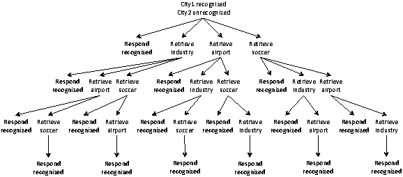
To give an example from the Model 1&3 class, Model 1&3.PN first reads
and encodes the city names. After these first steps, a race between
responding directly with the name of the recognized city (i.e., as in
Model 1) and retrieving and encoding one of the three cues (i.e., as in
Model 3.PN) takes place. If a retrieve-cue process wins, the retrieved
cue is encoded in the imaginal buffer and the race starts again. This
race is repeated either (a) until the model responds with the
recognized city before all three cues are retrieved (as in Model 1), or
(b) until all three cues are encoded and a decision is made in favor of
the recognized city (as in Model 3.PN).
As is explained in detail in Appendix C, in all race models, we assume
that the respond-with-recognized-city process (i.e., Model 1) competes
with all other processes of the respective simple model version (i.e.,
Model 3, Model 4, or Model 5). Consequently, the more steps that are
required prior to a decision being made, the more often the
respond-with-recognized-city process will compete against other
processes. To illustrate this, in the Model 1&4 class, the
respond-with-recognized-city process competes not only with the
retrieve-cue process, but, once all cues are retrieved, also with the
process of retrieving a big chunk (as in the Model 4 class).
Whereas in the Model 1&3 and 1&4 classes potentially all three cues
can be retrieved (i.e., if the respond-with-recognized-city process
does not win the race prior to retrieving all three cues), in the Model
1&5 class the number of cues that can be retrieved depends on the
decision criterion C. For example, in Model 1&5.1.PN, which
has a decision criterion of C = 1 positive or negative cue,
the respond-with-recognized-city process competes with the retrieve-cue
process until one positive or one negative cue has been retrieved. In
Model 1&5.2.PN (C = 2) and Model 1&5.3.PN (C = 3),
the race continues until two and three, respectively, positive or
negative cues have been retrieved. If a model of the Model 1&5 class
has retrieved all cues without reaching its decision criterion
C, it will use recognition as its best guess (as in the Model
5 class).
For all race models, we additionally implemented variants that not
only assume a race between noncompensatory recognition and
compensatory cue retrieval and usage, but additionally assume that
retrieved cues will at times be forgotten, such that these cues have
to be retrieved again. These models are marked with an F in
their name (e.g., Model 1&3.PN.F). The intuition is that the various
retrieval, encoding, and decision processes can detract from
previously retrieved cues (see Lewandowsky, Oberauer, & Braun, 2009,
for a discussion of interference based forgetting in working
memory). Specifically, these models start with a race between
responding with the recognized city and retrieving and encoding more
cues. As soon as at least two cues have been encoded in the imaginal
buffer, an additional race against a forgetting process takes
place.10 If this
forgetting process wins the race, the retrieved cues are forgotten
(i.e., they are removed from the imaginal buffer). If cues are
forgotten, then the race between responding with the recognized city
and retrieving and encoding cues takes place again. These processes
continue until a decision is made.
As can be seen in Table 2, the 1&4 and 1&5 race Model classes consist
of 8 and 12 different models, respectively. The large number of models
within these race model classes is a product of our principle of nested
modeling: Recall that the Model 4 class exists in two versions, L and
H, representing low and high activation levels of the big chunk.
Likewise, the Model 5 class exists in 3 versions, with each one making
different assumptions about the number of cues that will be processed
(i.e., C = 1, 2, or 3). To spare the reader from having to
parse long lists of model names, below we subsume the models from these
different versions of the Model 1&4 and 1&5 classes under the labels
Model 1&4.L and 1&4.H classes, as well as Model 1&5.1, 1&5.2, and
1&5.3 classes, respectively.
5 Description of the data analyses
5.1 Individual differences
It has been pointed out that people may differ in the strategies they
use when making decisions from the accessibility of memories (e.g.,
Bergert & Nosofsky, 2007; Bröder & Gaissmaier, 2007; Cokely,
Parpart, & Schooler, 2009; Gigerenzer & Brighton, 2009; Hilbig, 2008;
Marewski, Gaissmaier, Schooler, et al., 2009, 2010; B.R. Newell &
Shanks, 2004). For instance, Pachur et al. (2009) provided evidence
that processing speed influences people’s reliance on
recognition.
Also Pachur et al. (2008) interpreted their data as being suggestive
of individual differences: While some of their participants always
chose recognized cities irrespective of the cues they had been taught,
other participants’ decisions seemed to have been influenced by these
cues (see also Pachur, 2011). In reanalyzing Pachur et al.’s data, we
took possible individual differences into account by examining the
data separately for (a) those participants who always inferred
recognized cities to be larger than unrecognized ones (henceforth:
recognition group; nExperiment 1 =
25, nExperiment 2 = 19), and (b) those
participants who sometimes inferred unrecognized cities to be larger
(cue group; nExperiment 1 = 15,
nExperiment 2 = 21).
Moreover, we tailored the 39 models to each individual participant in
two steps. First, each participant’s responses in the recognition and
cue-memory tasks were used to model the contents of that participant’s
declarative memory. That is, we did not give the models perfect
knowledge of the cities and cue profiles as shown in Table 1 but
rather let the models operate on each individual participant’s
recognition and knowledge, as assessed by the recognition and
cue-memory tasks, respectively (see
http://www.ai.rug.nl/~katja/models or http://journal.sjdm.org/vol6.6.html for each participants’ knowledge
as used by the models). Second, using participants’ individual
recognition and cue knowledge, all models were run on each
participant’s trials in the decision task.
5.2 Assessing the correspondence between the models’
predictions and the human data
For simplicity and following the principle of nested modeling, we
assessed the correspondence between the models’ predictions and the
human data by analyzing these data in the same way Pachur et al.
(2008) analyzed the human data. Specifically, we collapsed the human
data across participants, calculating means and standard errors for
proportions (for decisions) as well as medians and the
1st and 3rd quartiles (for
decision times) separately for each of 2x3 categories of comparisons
of cities. In Experiment 1, these categories were: the recognized city
is associated with (a) one positive cue, (b) two positive cues, or (c)
three positive cues, and the recognized city is associated with (a)
two negative cues, (b) one negative cue, or (c) zero negative cues. In
Experiment 2, the 2x3 categories were: the recognized city is
associated with (a) zero, (b) two, or (c) three positive cues and with
(a) three, (b) one, or (c) zero negative cues. In both experiments,
the definition of the 2x3 categories was based on the cue profiles
participants had been taught in the learning tasks (Table
1).11
Decisions and decision times produced by the models could vary between
individual runs, due to noise and, where applicable, due to the race
between different processes. Therefore, to compute the
models’ predictions, for each participant of
Experiments 1 and 2, each model was run 40 times. For each of these 40
runs, we calculated means and standard errors as well as medians and
1st and 3rd quartiles, separately
for each of the 2x3 categories of each experiment in an analogous way
as for the human data. For each category, the means, standard errors,
medians, and quartiles were then averaged across the 40 simulation
runs.
5.3 Results of the model-fitting competition in
Experiment 1
Due to the large number of models, in what follows we will mainly
discuss the best models’ fits. All models’ fits are summarized in
Table 3 and discussed in more detail in Appendix B. Appendix B also
includes a complete set of graphs of all models’ fits.
| Table 3: Root mean square deviations (RMSDs) between the model
and the human data in Experiment 1 |
| | Recognition group | Cue group |
| | Decisions (%) | Decision times (ms) | Decisions (%) | Decision times (ms) |
| Model 1 class: Stopping and
decision rules noncompensatory—simple model |
| Model 1 | 0 | 409 | 9.4 b | 511 |
| Model 2 class: Stopping rule
compensatory, decision rule noncompensatory—simple models |
| Model 2.PN | 0 | 258 | 9.4 b | 355 |
| Model 2.P | 0 | 283 | 9.4 b | 376 |
| Model 3 class: Stopping rule
compensatory, decision rule noncompensatory—simple models |
| Model 3.PN | 0 | 357 | 9.4 b | 449 |
| Model 3.P | 0 | 379 | 9.4 b | 469 |
| Model 1&3 class: Stopping rule
noncompensatory and compensatory, decision rule noncompensatory—race models |
| Model 1&3.PN | 0 | 110 | 9.4 b | 219 |
| Model 1&3.P | 0 | 97 | 9.4 b | 201 |
| Model 1&3.PN.F | 0 | 73 | 9.4 b | 185 |
| Model 1&3.P.F | 0 | 67 | 9.4 b | 169 |
| Model 4 class: Stopping rule
compensatory, decision rule compensatory—simple models |
| Model 4.H.PN | 10.7 a | 427 | 0.9 | 499 |
| Model 4.H.P | 10.7 a | 477 | 1.5 | 518 |
| Model 4.L.PN | 58.6 a | 461 | 49.4 | 514 |
| Model 4.L.P | 59.1 a | 511 | 49.6 | 534 |
| Model 1&4 class: Stopping rule
noncompensatory and compensatory, decision rule noncompensatory and compensatory—race
models |
| Model 1&4.H.PN | 1.3 a | 105 | 8.1 | 223 |
| Model 1&4.H.P | 1.3 a | 100 | 8.1 | 198 |
| Model 1&4.H.PN.F | .8 a | 71 | 8.5 | 177 |
| Model 1&4.H.P.F | .7 a | 55 | 8.6 | 157 |
| Model 1&4.L.PN | 7.3 a | 109 | 1.9 | 218 |
| Model 1&4.L.P | 7.3 a | 95 | 2.1 | 197 |
| Model 1&4.L.PN.F | 4.2 a | 63 | 5.1 | 176 |
| Model 1&4.L.P.F | 4.3 a | 56 | 5.1 | 155 |
| Model 5 class: Stopping rule
compensatory, decision rule compensatory—simple models |
| Model 5.1.PN | 40.7 a | 259 | 32.4 | 389 |
| Model 5.1.P | 0 | 193 | 9.4 b | 286 |
| Model 5.2.PN | 48.1a | 304 | 39.5 | 395 |
| Model 5.2.P | 0 | 352 | 9.4 b | 431 |
| Model 5.3.PN | 0 | 357 | 9.4 b | 449 |
| Model 5.3.P | 0 | 379 | 9.4 b | 469 |
| Model 1&5 class: Stopping rule
noncompensatory and compensatory, decision rule noncompensatory and compensatory—race
models |
| Model 1&5.1.PN | 15 a | 243 | 8.3 | 372 |
| Model 1&5.1.P | 0 | 209 | 9.4 b | 326 |
| Model 1&5.1.PN.F | 15.1 a | 244 | 8.1 | 370 |
| Model 1&5.1.P.F | 0 | 205 | 9.4 b | 324 |
| Model 1&5.2.PN | 8.1 a | 133 | 6.8 | 248 |
| Model 1&5.2.P | 0 | 118 | 9.4 b | 220 |
| Model 1&5.2.PN.F | 5.7 a | 106 | 6.8 | 212 |
| Model 1&5.2.P.F | 0 | 96 | 9.4 b | 189 |
| Model 1&5.3.PN | 0 | 109 | 9.4 b | 223 |
| Model 1&5.3.P | 0 | 97 | 9.4 b | 203 |
| Model 1&5.3.PN.F | 0 | 75 | 9.4 b | 188 |
| Model 1&5.3.P.F | 0 | 70 | 9.4 b | 167 |
| Note. PN = Positive and negative cues. P = Positive cues. F =
Forgetting cues. For decisions, RMSDs were calculated on the mean
percentage of choices for the recognized city. For models that always
decide for the recognized city, RMSDs for decisions will–by
definition—always be 0 in the recognition group. For decision times,
RMSDs were calculated on the median and the 1st and 3rd quartile and
then averaged. Evaluations of the models’ fit based on
RMSDs should be complemented by visual inspections of the data produced
by the models (see Figures 5–8 and Appendix B: Figures B1-B18). |
| a These models do by definition not fit the decision
of the recognition group, because they sometimes decide for the
unrecognized city whereas participants in the recognition group always
decide for the recognized city. |
| b These models do by definition not fit the decision
of the cue group, because they always decide for the recognized city
whereas participants in the cue group sometimes decide for the
unrecognized city. |
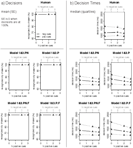
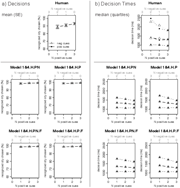
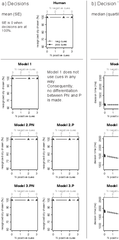
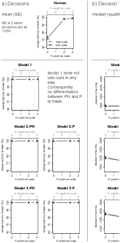
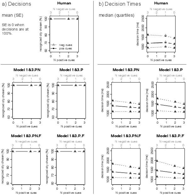
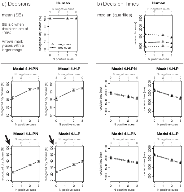
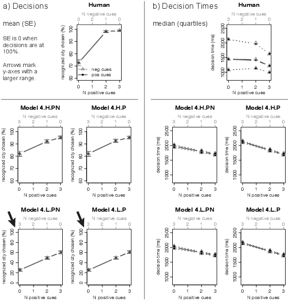
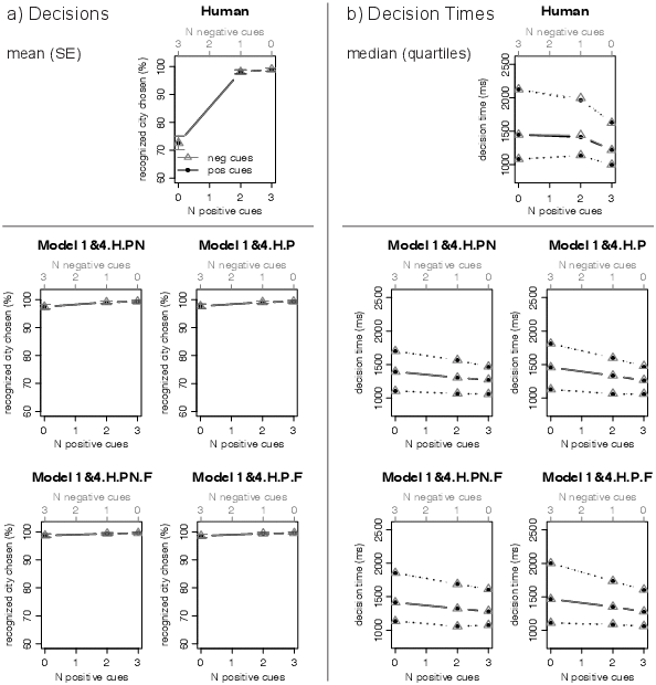
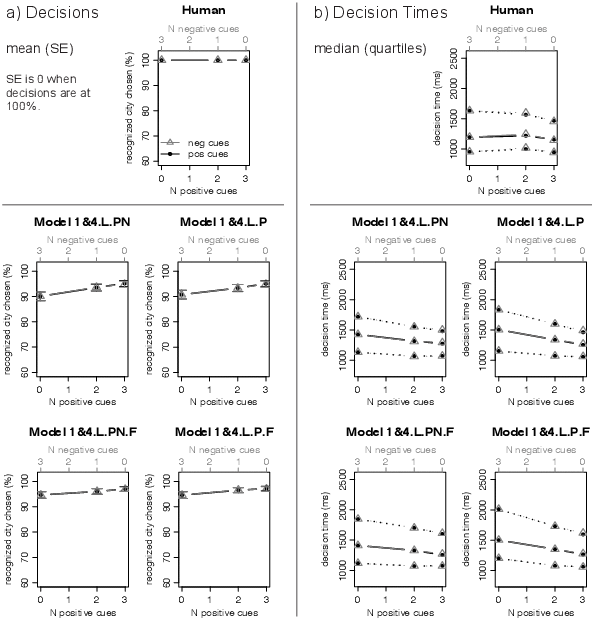
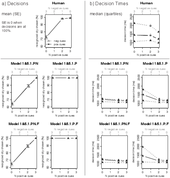
| Figure 5: Decisions (a) and decision times (b) for the
recognition group in Experiment 1. Human data and fits of the four
models from the Model 1&3 class. Models are ordered from the top left
to the bottom right in the same order as in Tables 2, 3, and 4. In each
graph, the upper grey x-axis shows the number of negative cues; the
corresponding data points (decisions in Panel A, decision times in
Panel B) are plotted in grey font (triangles). In each graph, the lower
black x-axis shows the number of positive cues; the corresponding data
points are plotted in black font (circles). For instance, in Panel B
the median of the human decision times is 1335 ms for two negative cues
and 1332 ms for one positive cue. |

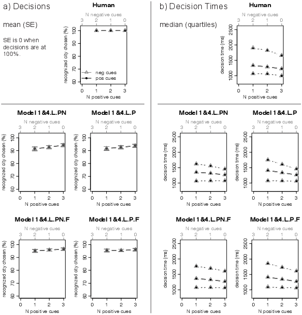
| Figure 6: Decisions (a) and decision times (b) for
the recognition group in Experiment 1. Human data and fits of those six
models from the Model 1&5.2 and 1&5.3 classes that always decide for
the recognized city in Experiment 1. Models are ordered from the top
left to the bottom right in the same order as in Tables 2, 3, and 4. In
each graph, the upper grey x-axis shows the number of negative cues;
the corresponding data points (decisions in Panel A, decision times in
Panel B) are plotted in grey font (triangles). In each graph, the lower
black x-axis shows the number of positive cues; the corresponding data
points are plotted in black font (circles). |

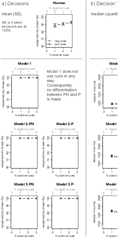
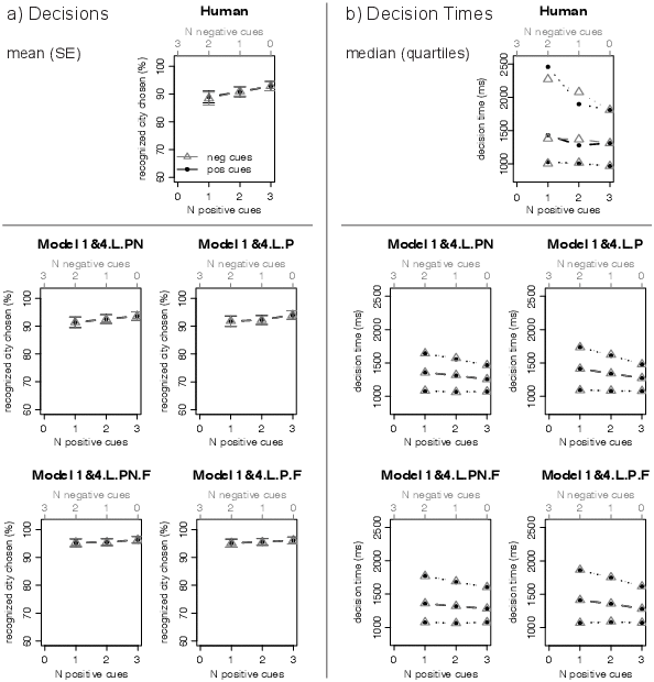
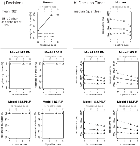
| Figure 7: Decisions (A) and decision times (B) for the
cue group in Experiment 1. Human data and fits of the four models from
the Model 1&4.L class. Models are ordered from the top left to the
bottom right in the same order as in Tables 2, 3, and 4. In each graph,
the upper grey x-axis shows the number of negative cues; the
corresponding data points (decisions in Panel A, decision times in
Panel B) are plotted in grey font (triangles). In each graph, the lower
black x-axis shows the number of positive cues; the corresponding data
points are plotted in black font (circles). For instance, in Panel A
the mean percentage of participants’ choices for the
recognized city is 88 for two negative cues and 89 for one positive
cue. |

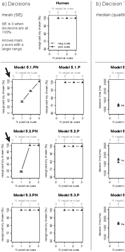
| Figure 8: Decisions (A) and decision times (B) for the cue group in
Experiment 1. Human data and fits of those two models from the
Model 1&5.2 class that sometimes decide against the recognized
city in Experiment 1. Models are ordered from left to right in the
same order as in Tables 2, 3, and 4. In each graph, the upper grey
x-axis shows the number of negative cues; the corresponding data
points (decisions in Panel A, decision times in Panel B) are
plotted in grey font (triangles). In each graph, the lower black
x-axis shows the number of positive cues; the corresponding data
points are plotted in black font (circles). |

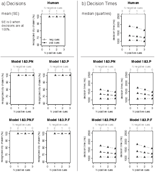
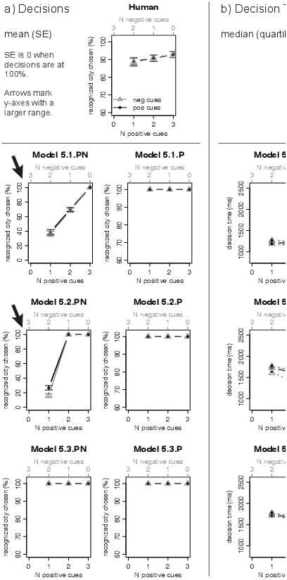
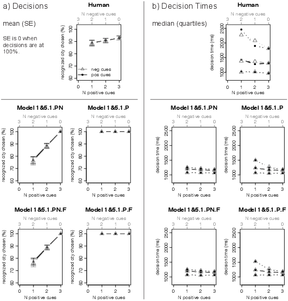
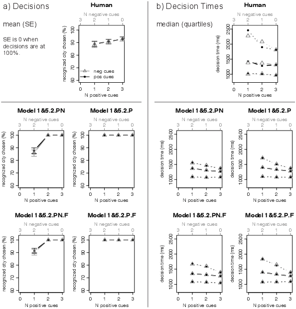
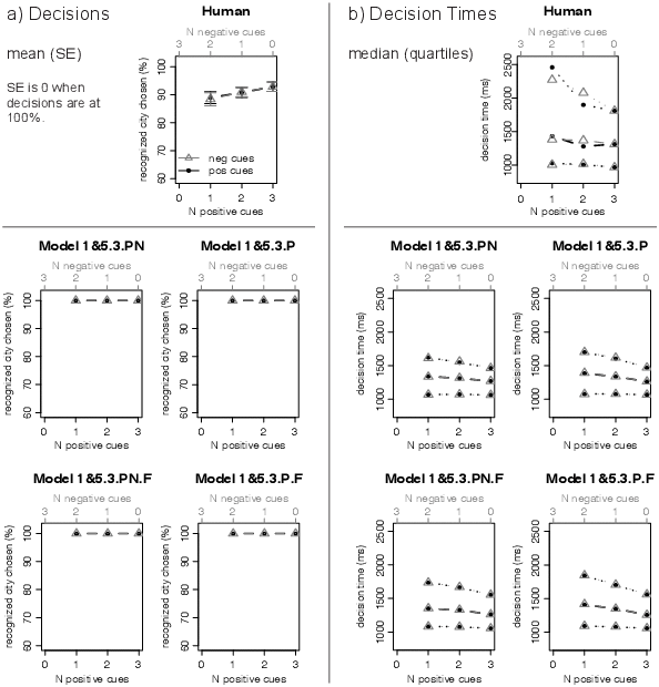
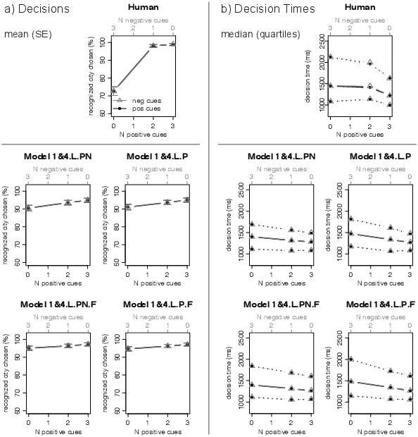
Recognition group. Figure 5 shows the human decisions and
decision times in the recognition group as well as the decisions and
decision times produced by the Model 1&3 class. Within this model
class, Model 1&3.P.F produced the smallest RMSDs to the human
data. As can be seen, neither the human decisions nor the model’s
decisions vary as a function of the cues. At the same time, the human
and the model’s decision times increase with the number of negative
cues, decrease with the number of positive cues and show overall a
large spread. Also the three remaining models of the 1&3 class,
Models 1&3.PN, 1&3.PN.F, and 1&3.P, fit the decisions and decision
times well. These three models are identical to Model 1&3.P.F except
that they make no assumptions about the forgetting of cues (Models
1&3.PN, 1&3.P) and/or assume negative cues to be represented in
memory (Models 1&3.PN, 1&3.PN.F).
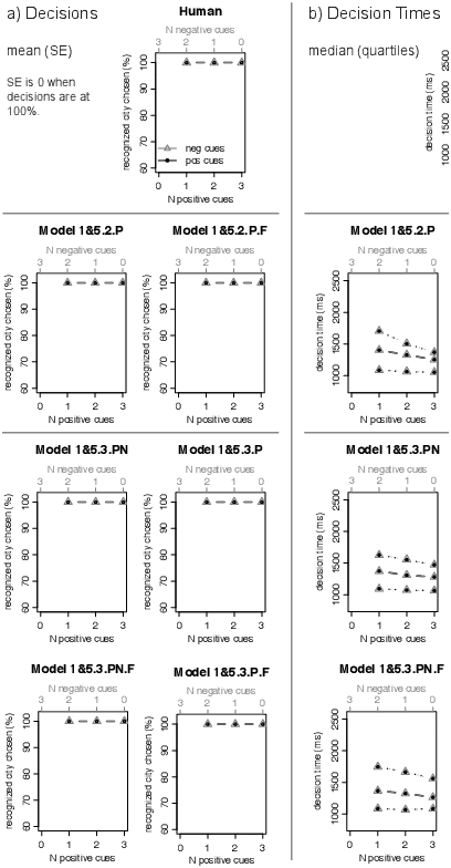
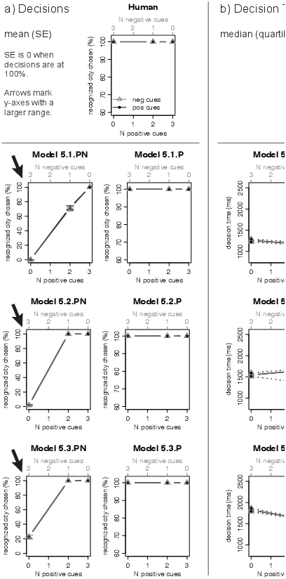
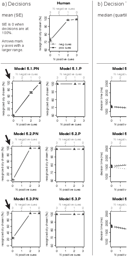
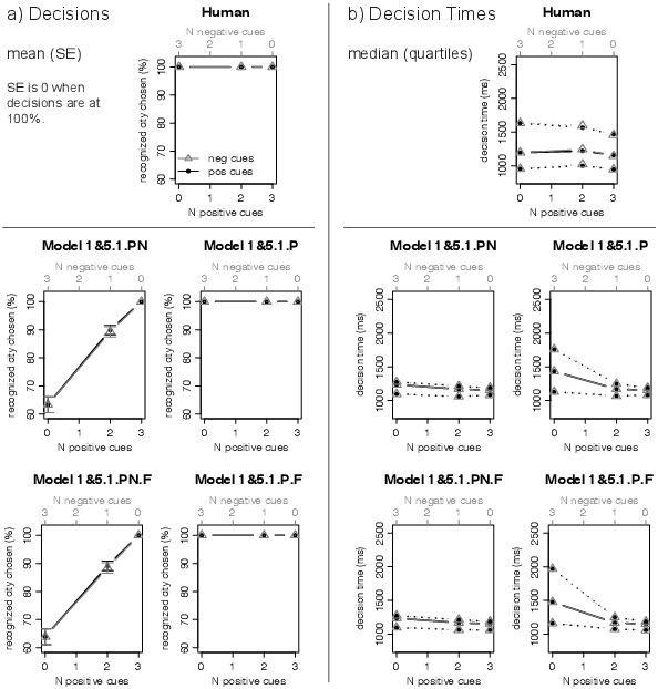
As can be seen in Table 3 as well as by comparing Figures 5 and 6, those
representatives of the Model 1&5 class that assume a decision
criterion of 3 cues (Model 1&5.3.PN, Model 1&5.3.PN.F, Model
1&5.3.P, Model 1&5.3.P.F) fit the decisions and decision times
about as well as the Model 1&3 class. For example, the best-fitting
model from the Model 1&5.3 class, Model 1&5.3.P.F, produces basically
the same decision time pattern as the best-fitting model from the Model
1&3 class, Model 1&3.P.F, and virtually the same RMSDs. Also those
representatives of the Model 1&5 class that assume a decision
criterion of 2 positive cues (Model 1&5.2.P, 1&5.2.P.F) fit the
decisions and decision times well.
Importantly, while technically (i.e., by virtue of their
RMSDs) Models 1&3.P.F and 1&5.3.P.F are the best-fitting models in
Experiment 1’s recognition group, the models of the 1&3 and 1&5.3
classes, as well as the P versions of the Model 1&5.2 class produce
relatively similar fits. Therefore, we caution to declare any specific
model from these classes to be considered the single winner. Rather,
we would prefer to consider these classes the winner. In short, in
Experiment 1’s recognition group, the best-fitting model classes
implement a race between Model 1’s recognition-based noncompensatory
stopping and decision rules and other processes; namely (i) Model 3’s
compensatory stopping rule and its recognition-based noncompensatory
decision rule (i.e., as in the Model 1&3 class) as well as (ii) Model
5’s compensatory stopping and decision rules (i.e., as in the Model
1&5 class).
We would like to add three observations with respect to the Model 1&5
class. First, note that Model 1&5.3.PN’s and Model 1&5.3.PN.F’s
comparatively good fit of the recognition group’s decisions (Figure 6)
can be explained by Experiment 1’s design. These two models need to
retrieve 3 negative cues to decide against the recognized city
(C = 3). As 3 negative cues were not taught in Experiment
1 (Table 1), Model 1&5.3.PN and Model 1&5.3.PN.F could not reach
this decision criterion in Experiment 1, resulting in the models to
always decide in favor of recognized cities. Had 3 negative cues been
taught in Experiment 1, Model 1&5.3.PN and Model 1&5.3.PN.F would
have produced decisions in favor of unrecognized cities, resulting in
poor fits in the recognition group.12
Second, while one could thus argue that Model 1&5.3.PN’s and Model
1&5.3.PN.F’s good fit is an artifact of Experiment 1’s design, the
comparatively good fit of Model 1&5.3.P and Model 1&5.3.P.F is no
such artifact: As these two models do not use negative cue knowledge,
they never decide against unrecognized cities, but use recognition and
positive cues to decide in favor of recognized ones. On the other
hand, one may wonder whether compensatory, cue-based models that can
never decide against unrecognized objects are theoretically
plausible, or, what such models would add beyond models with simpler
recognition-based, noncompensatory decision rules (e.g., as
implemented by the Model 1&3 class).
Third, also Models 1&5.1.P and 1&5.1.P.F which assume a decision
criterion C of 1 positive cue exhibit relatively small RMSDs
(Table 3). By this token, also these representatives of the Model 1&5
class may belong to the winners. However, note that Models 1&5.1.P
and 1&5.1.P.F produce a much smaller spread in the decision time
distribution than the spread that can be found in the human times
(Figure B13 in Appendix B).
Cue group. Figure 7 shows the human decisions and decision
times as well as the decisions and decision times produced by the
Model 1&4.L class, which is the class that best fits the combination
of decisions and decision times in the cue group. As can be seen, the
human decisions and decision times as well as the models’ decisions
and decision times vary as a function of cues. The decision times
show a large spread. While the Model 1&4.L class emerges as the
best-fitting class, it is difficult to rank order the models
within that class in terms of their RMSDs. As Table 3 shows,
Model 1&4.L.P.F fits the decision times best; however, this model
does not produce the smallest RMSDs for the decisions, which are
produced by Model 1&4.L.PN.
Let us turn to a couple of other models that may, perhaps, be
considered to belong to the winners in the cue group. First, as can be
seen in Table 3, the Model 1&4.H class, which differs from the Model
1&4.L class only in the base level activation of the big-chunk,
produces a good fit of the decision times, while not fitting the
decisions as well as the 1&4.L class (Figure B8 in Appendix
B). Second, Table 3 suggests that also the PN versions of the Model
1&5.2 class (i.e., Model 1&5.2.PN, 1&5.2.PN.F) produce a relatively
good fit to the cue group’s combination of decisions and decision
times. However, as a visual inspection of Figure 8 reveals, these
models produce an abrupt drop in decisions for the recognized city as
soon as the decision criterion of C = 2 negative cues is
reached. The human data do not exhibit such a drop. Much the same can
be said with respect to the PN versions of the Model 1&5.1 class
(Figure B13 in Appendix B), which produce an even steeper drop in the
decisions, and which fit the spread of the decision times less well
than the Model 1&5.2 class.
In short, the cue group’s best-fitting models are members of the Model
1&4.L class. This model class implements a race between Model 1’s
noncompensatory stopping rule and Model 4’s compensatory stopping rule
as well as a race between Model 1’s noncompensatory decision rule and
Model 4’s compensatory decision rule, assuming implicit, intuitive
knowledge about the cities’ sizes to be responsible for occasional
decisions in favor of unrecognized cities.
5.4 Results of the model generalization competition in
Experiment 2
To test how well these results generalize to another data set, we let
all 39 models predict the human decisions and decision times from
Experiment 2. In doing so, we populated the models’ declarative memory
with each individual participant’s recognition and cue knowledge,
using participants’ responses in the recognition task and cue-memory
task of Experiment 2—just as we did in Experiment 1. And as in
Experiment 1, we ran the models on the trials of each individual
participant in the decision task of Experiment 2. Following our
principle of predictive modeling, we kept all models’ production rules
as well as the values of all models’ parameters identical to those
used in Experiment 1.
| Table 4: Root mean square deviations (RMSDS) between the model and the
human data in Experiment 2 |
| | Recognition group | Cue group |
| | Decisions (%) | Decision times (ms) | Decisions (%) | Decision times (ms) |
| Model 1 class: Stopping and
decision rules noncompensatory—simple model |
| Model 1 | 0 | 279 | 15.9 b | 498 |
| Model 2 class: Stopping rule
compensatory, decision rule noncompensatory—simple models |
| Model 2.PN | 0 | 255 | 15.9 b | 290 |
| Model 2.P | 0 | 307 | 15.9 b | 320 |
| Model 3 class: Stopping rule
compensatory, decision rule noncompensatory—simple models |
| Model 3.PN | 0 | 454 | 15.9 b | 380 |
| Model 3.P | 0 | 531 | 15.9 b | 410 |
| Model 1&3 class: Stopping rule
noncompensatory and compensatory, decision rule noncompensatory—race models |
| Model 1&3.PN | 0 | 101 | 15.9 b | 170 |
| Model 1&3.P | 0 | 135 | 15.9 b | 145 |
| Model 1&3.PN.F | 0 | 134 | 15.9 b | 131 |
| Model 1&3.P.F | 0 | 179 | 15.9 b | 109 |
| Model 4 class: Stopping rule
compensatory, decision rule compensatory—simple models |
| Model 4.H.PN | 11.7 a | 590 | 6.8 | 435 |
| Model 4.H.P | 12 a | 666 | 6.6 | 474 |
| Model 4.L.PN | 57.8 a | 623 | 45.1 | 456 |
| Model 4.L.P | 57.1 a | 699 | 44.9 | 500 |
| Model 1&4 class: Stopping rule
noncompensatory and compensatory, decision rule noncompensatory and compensatory—race
models |
| Model 1&4.H.PN | 1.6 a | 100 | 14.4 | 164 |
| Model 1&4.H.P | 1.6 a | 151 | 14.5 | 140 |
| Model 1&4.H.PN.F | 0.9 a | 138 | 15.1 | 124 |
| Model 1&4.H.P.F | 0.8 a | 180 | 15.1 | 88 |
| Model 1&4.L.PN | 7.4 a | 115 | 10.9 | 166 |
| Model 1&4.L.P | 7.2 a | 150 | 11.2 | 145 |
| Model 1&4.L.PN.F | 4.2 a | 147 | 13.1 | 125 |
| Model 1&4.L.P.F | 4 a | 204 | 12.9 | 95 |
| Model 5 class: Stopping rule
compensatory, decision rule compensatory—simple models |
| Model 5.1.PN | 60.1 a | 193 | 44.8 | 331 |
| Model 5.1.P | 0 | 436 | 15.9 b | 409 |
| Model 5.2.PN | 56.7 a | 284 | 40.8 | 295 |
| Model 5.2.P | 0 | 472 | 15.9 b | 373 |
| Model 5.3.PN | 44.7 a | 453 | 28.5 | 380 |
| Model 5.3.P | 0 | 531 | 15.9 b | 410 |
| Model 1&5 class: Stopping rule
noncompensatory and compensatory, decision rule noncompensatory and compensatory—race
models |
| Model 1&5.1.PN | 22 a | 166 | 7.2 | 321 |
| Model 1&5.1.P | 0 | 177 | 15.9 b | 251 |
| Model 1&5.1.PN.F | 21.8 a | 163 | 6.9 | 320 |
| Model 1&5.1.P.F | 0 | 208 | 15.9 b | 236 |
| Model 1&5.2.PN | 13 a | 123 | 2.9 | 206 |
| Model 1&5.2.P | 0 | 142 | 15.9 b | 167 |
| Model 1&5.2.PN.F | 10.5 a | 106 | 5.6 | 185 |
| Model 1&5.2.P.F | 0 | 175 | 15.9 b | 131 |
| Model 1&5.3.PN | 5.8 a | 99 | 10.2 | 162 |
| Model 1&5.3.P | 0 | 146 | 15.9 b | 146 |
| Model 1&5.3.PN.F | 3.1 a | 131 | 12.6 | 135 |
| Model 1&5.3.P.F | 0 | 167 | 15.9 b | 104 |
| Note. PN = Positive and negative cues. P = Positive
cues. F = Forgetting cues. For decisions, RMSDs were calculated on the
mean percentage of choices for the recognized city. For models that
always decide for the recognized city, RMSDs for decisions will—by
definition—always be 0 in the recognition group. For decision times,
RMSDs were calculated on the median and the 1st and 3rd quartile and
then averaged. Evaluations of the models’ fit based on
RMSDs should be complemented by visual inspections of the data produced
by the models (see Figures 9–12, and Appendix B: Figures B19-B36). |
| a These models do by definition not fit the decision
of the recognition group, because they sometimes decide for the
unrecognized city whereas participants in the recognition group always
decide for the recognized city. |
| b These models do by definition not fit the decision
of the cue group, because they always decide for the recognized city
whereas participants in the cue group sometimes decide for the
unrecognized city. |
| Figure 9: Decisions (A) and decision times (B) for the
recognition group in Experiment 2. Human data and predictions of the
four models from the Model 1&3 class. Models are ordered from the top
left to the bottom right in the same order as in Tables 2, 3, and 4. In
each graph, the upper grey x-axis shows the number of negative cues;
the corresponding data points (decisions in Panel A, decision times in
Panel B) are plotted in grey font (triangles). In each graph, the lower
black x-axis shows the number of positive cues; the corresponding data
points are plotted in black font (circles). |

| Figure 10: Decisions (A) and decision times (B) for the
recognition group in Experiment 2. Human data and predictions of those
four models from the Model 1&5.2 and 1&5.3 classes that always decide
for the recognized city in Experiment 2. Models are ordered from the
top left to the bottom right in the same order as in Tables 2, 3, and
4. In each graph, the upper grey x-axis shows the number of negative
cues; the corresponding data points (decisions in Panel A, decision
times in Panel B) are plotted in grey font (triangles). In each graph,
the lower black x-axis shows the number of positive cues; the
corresponding data points are plotted in black font (circles). |

Table 4 summarizes the results for all models. In what follows,
we will mainly discuss those models that generalized best (for all
other models’ generalizability and a complete set of
graphs of all models’ predictions see Appendix B.)
| Figure 11: Decisions (A) and decision times (B) for the cue
group in Experiment 2. Human data and predictions from the four models
from the Model 1&4.L class. Models are ordered from the top left to
the bottom right in the same order as in Tables 2, 3, and 4. In each
graph, the upper grey x-axis shows the number of negative cues; the
corresponding data points (decisions in Panel A, decision times in
Panel B) are plotted in grey font (triangles). In each graph the lower
black, x-axis shows the number of positive cues; the corresponding data
points are plotted in black font (circles). |

| Figure 12: Decisions (A) and decision times (B) for the cue
group in Experiment 2. Human data and predictions from those four
models from the Model 1&5.2 and 1&5.3 classes that sometimes decide
against the recognized city in Experiment 2. Models are ordered from
the top left to the bottom right in the same order as in Tables 2, 3,
and 4. In each graph, the upper grey x-axis shows the number of
negative cues; the corresponding data points (decisions in Panel A,
decision times in Panel B) are plotted in grey font (triangles). In
each graph the lower black, x-axis shows the number of positive cues;
the corresponding data points are plotted in black font (circles). |

Recognition group. Figures 9 and 10 show the human decisions
and decision times as well as the corresponding data produced by the
best-generalizing models in the recognition group. These are
representatives of the Model 1&3 class, as well as those
representatives from the Model 1&5 class that assume a decision
criterion of 2 and 3 positive cues (Models 1&5.2.P, 1&5.2.P.F,
1&5.3.P, 1&5.3.P.F). As can be seen, all winning models correctly
predict that decisions do not vary as a function of cues. The models
also predict the overall pattern and spread of the decision times well.
Importantly, as the RMSDs in Table 4 show, the technically
best-generalizing model, Model 1&3.PN, belongs to the Model 1&3
class, which also was one of the winning model classes in Experiment 1,
lending, perhaps, further support to the 1&3 class.
Note that also Model 1&5.1.P—and to a lesser extent Model
1&5.1.P.F—exhibit relatively small RMSD in Table 4. However, as in
Experiment 1, these models fail to predict the spread of the human
decision times (Figure B31 in Appendix B).
In short, for the recognition group, members of the Model 1&3 class
are among the best models in both experiments. Also the versions of
the Model 1&5.2 and 1&5.3 class that use only positive cues perform
well in both experiments. The versions of the Model 1&5.3 class that
use positive and negative cues fitted Experiment 1’s
recognition group well (Figure 6), but do not predict the
recognition group’s decisions in Experiment 2. Recall that these two
models need to retrieve 3 negative cues to decide against the
recognized city. As 3 negative cues were not taught in Experiment 1
(Table 1), the models did not reach their decision criterion,
leading them to always decide in favor of recognized cities. In
Experiment 2, in contrast, 3 negative cues were taught.
Correspondingly, the models do reach their decision criterion, leading
them to occasionally decide against the recognized city, this way
mismatching the recognition group data. However, as we explain next,
the models turn out to generalize well to Experiment 2’s cue group.
Cue group. Figures 11 and 12 show the human data and the
best-generalizing models in the cue group. These are the Model 1&4.L
class as well as those representatives of the Model 1&5.2 and 1&5.3
classes that use positive and negative cues.
Let us first turn to the decisions of the Model 1&4.L class, which
fitted the data best in Experiment 1. As in Experiment 1, the human
decisions, as well as the decisions of the models vary as a function of
cues. However, in Experiment 2, the human decisions are strongly
influenced by three negative cues (i.e., corresponding to zero positive
cues). Having been adjusted to Experiment 1, in which participants were
taught a maximum of two negative cues (Table 1), the Model 1&4.L
class fits the decisions for zero and one negative cue well, but has
difficulties to predict the large effect of three negative cues in
Experiment 2 (Figure 11). Much the same can be said with respect to the
Model 1&4.H class, which, as in Experiment 1, does not predict the
decisions as well as the 1&4.L class (Table 4; Figure B26 in Appendix
B).
In contrast, consider the decisions of the PN versions of the Model
1&5.2 and 1&5.3 classes (Model 1&5.2.PN, 1&5.2.PN.F, 1&5.3.PN,
1&5.3.PN.F). As shown in Figure 12, these models do predict a
large effect of negative cues on the decisions once their decision
criterion of C negative cues is reached. Models 1&5.2.PN and
1&5.2.PN.F, which decide against the recognized city as soon as two
negative cues have been retrieved, predict the pattern in the human
decisions best (Table 4, Figure 12).
Figures 11 and 12 also show the decision times. The models from the
1&4.L class as well as the PN versions of the 1&5.2, and 1&5.3
classes are able to approximate the human decision time pattern and its
spread. However, Models 1&5.2.PN and 1&5.2.PN.F, which predict the
decisions best, do not predict the decision times as well as the
representatives of the 1&4.L class and the PN versions of the 1&5.3
class (Table 4), making it difficult to rank the best model
classes in terms of their performance.
Note that, as in Experiment 1, also the PN versions of the Model
1&5.1 class produce a drop in the decisions once its decision
criterion of C = 1 negative cues is reached. However, this
drop is steeper than in the human data and the model class fails to
predict the spread of the decision times (Figure B32 in Appendix B.)
In short, the winning model classes in Experiment 2’s cue group are
essentially identical to those that won in Experiment 1’s cue
group—with two relevant caveats. First, in Experiment 2, besides the
Model 1&4.L and 1&4.H classes, and the PN versions of the 1&5.2
classes, also the PN versions of the Model 1&5.3 class may be
considered to belong to the winners. Second, in Experiment 1, the
Model 1&4.L class fitted the decisions and decision times best. In
Experiment 2, it is more difficult to establish a rank order of these
classes’ ability to predict the human data, as those models that
predict the decisions best do not predict the decision times
best.13
6 General discussion
Much research has investigated how people make decisions based on a
sense of the accessibility of memories, as assumed by the recognition
heuristic and related models (Bruner, 1957; Jacoby & Dallas,
1981; Pachur et al., 2011; Pohl, 2011; Tversky & Kahneman, 1973). At
the same time, in the field of accessibility-based decision making and
beyond, many have criticized the lack of specification of process
hypotheses (e.g., Dougherty et al., 1999, 2008; Gigerenzer, 1996; 1998;
Keren & Schul, 2009; A. Newell, 1973). Particularly the recognition
heuristic has triggered a controversy about what processes describe
people’s decisions best when they make inferences from
the accessibility of memories: Do people rely on this noncompensatory
heuristic, ignoring further knowledge, or do they use compensatory
strategies instead?
In this article, we provided a primer on how the precision of
corresponding process hypotheses can be increased. Using the ACT-R
cognitive architecture, we specified process hypotheses about
accessibility-based decisions in 39 quantitative process models. These
models do not only capture decision processes, but also the interplay
of decision processes with perceptual, memory, intentional, and motor
processes. Moreover, by implementing a number of decision models that
had originally been defined at different levels of description into
one architectural modeling framework, we made these models
comparable, providing a basis for detailed, multi-experiment model
comparisons to be conducted in future research. Finally, we conducted a
first model comparison ourselves, re-analyzing two previously published
data sets.
Even though the main objective of this model comparison was to
illustrate how such comparisons can be conducted rather than to
conclusively identify the best model, in what follows we will first
discuss our model comparison’s results. We will close
by turning to a number of broader methodological issues.
6.1 Dissolving dichotomies by implementing more than one
process: Race models
Both in fitting existing data and in generalizing to new data,
representatives of the race model classes performed best in our model
competition. As such, the winners are models that implement
recognition-based noncompensatory processes side by side with
cue-based compensatory ones, suggesting that in one part of the trials
in the decision task noncompensatory processes governed information
retrieval and/or decision making, while in the other part compensatory
processes were dominant. Specifically, our results highlight the
possibility that even people who always responded with recognized
cities (i.e., as in the recognition group) most likely retrieved and
encoded cues in at least some of the trials. People who sometimes
responded with unrecognized cities (i.e., as in the cue group), in
turn, most likely based their decisions on cues in some of the trials
but ignored these cues and relied on recognition in others. These
results let the dichotomy between cue-based compensatory and
recognition-based noncompensatory processes dissolve that is often
assumed in the literature and that has fuelled debates about the
recognition heuristic (e.g., Pohl, 2006, 2011; Richter & Späth,
2006; see above). Moreover, these results cast, perhaps, some doubt
on a simplifying assumption that is central to this debate: By
classifying a person exclusively as either a noncompensatory or a
compensatory decision maker, previous studies had (at least
implicitly) assumed that a person’s decision processes do not vary
across the trials of a decision task (e.g., Glöckner & Bröder,
2011; Marewski, Gaissmaier, Schooler, et al., 2010).14
We hasten to add that our analyses entailed collapsing the data across
participants’ responses, which severely limits the possibility to draw
conclusions about individual persons’ decision processes. We suggest
for future research to tackle this question, by using more exhaustive
human data sets and analyses.
6.2 Models implementing one decision process: Simple models
Models that implement merely one type of decision process, namely
noncompensatory or compensatory, did not account as well for
people’s behavior as the winning race models. Let us
first turn to the noncompensatory models, and then to the compensatory
ones.
Noncompensatory models. The strictly noncompensatory Model
1, which neither retrieves nor uses cues for decisions, did not
accurately predict participants’ decision times, even for participants
who always chose the recognized city (Appendix B, Figures B1, B19). As
such, our results cast doubts on recognition heuristic implementations
that assume noncompensatory recognition-based stopping and decision
rules. Much the same can be said with respect to those recognition
heuristic implementations that retrieve cues but do not use them for
decisions: Also the Model 2 and 3 classes, which implement
corresponding cue-based compensatory stopping and recognition-based
noncompensatory decision rules, did not account well for people’s
behavior (Appendix B, Figures B1, B19). However, the relative success
of the 1&3 race Model class lends support to a combination
of both recognition heuristic implementations: As the Model 1&3 class
includes Model 1 and Model 3 as components, our results
suggest that a combination of these two recognition heuristic
implementations may reflect people’s decision processes in the
comparisons of cities (Gigerenzer & Goldstein, 2011).
We would like to add two points. First, while representatives of the
Model 1&3 class are both among Experiment 1’s best fitting and among
Experiment 2’s best generalizing models, also those representatives of
the 1&5 Model class that rely on positive cues in addition to
recognition were able to account for behavior well. This result leads
us to stress that it may be similarly plausible for noncompensatory,
recognition-based stopping and decision rules to govern a part of the
comparisons of two cities (i.e., Model 1), while compensatory,
cue-based processes govern the other part (i.e., Model 5). On the
other hand, the Model 1&3 class provides, arguably, a simpler
explanation for the human data than the Model 1&5 class.
Second, we implemented just one strictly noncompensatory
variant of the recognition heuristic: Model 1, which has both
a recognition-based noncompensatory stopping and decision
rule. It is to be expected that pitting this single strictly
noncompensatory model against a total of 38 other models may have
biased the outcome of the model comparison against strictly
noncompensatory models.
Compensatory models. We implemented two types of strictly
compensatory models. In assuming that subsymbolic pathways and
spreading activation give rise to implicit, intuitive knowledge that
governs compensatory decision processes, the Model 4 class implements a
central feature of Glöckner and Betsch’s (2008)
parallel constraint satisfaction model. The parallel constraint
satisfaction model has been argued to account for behavior better than
the recognition heuristic—at times without the model having been
applied to data (e.g., Hilbig & Pohl, 2009; Hochman, et al, 2010; see
Glöckner & Bröder, 2011, for a test that does apply the model to
data).
The Model 5 class assumes symbolic pathways to be responsible for
compensatory processes, and as such, decisions to be based on explicit,
deliberate knowledge. Also models from this class have been discussed
as antipodes to the recognition heuristic; almost always with such
models not being applied to data (e.g., Hilbig & Pohl, 2009; B. R.
Newell & Shanks, 2004; Oeusoonthornwattana & Shanks, 2010; Pohl,
2006; Richter & Späth, 2006), or with the models having been applied
to data, but without using the models to quantitatively predict
decision times (Marewski, Gaissmaier, Schooler, et al., 2009; Pachur &
Biele, 2007).
Whereas both Model 4 and Model 5 classes were able to account for some
aspect of the human data in the cue group, neither turned out to be
sufficient (Appendix B; Figures B6, B12, B24, B30). Instead, the
race models of the Model 1& 4 class, that is, combinations of the
implicit, intuitive processes assumed by Model 4 and the
noncompensatory, recognition-based processes of Model 1 were able to
fit participant’s data best in Experiment 1. In
Experiment 2, race models of the 1&4 class were also among the
best-generalizing models; however, here representatives of the Model
1&5 class rivaled their performance. In short, with respect to
strictly compensatory models, the current data suggest that the simple
Model 4 and 5 classes are insufficient.
6.3 Methodological considerations
Model specification. At the close of this article, we would
like to stress five points. First, most of the hypotheses about
accessibility-based decisions tested here had only been formulated
verbally in the literature. As a result, the outcomes of our model
comparison also depend on our choices of how to implement such verbal
hypotheses into detailed computational models in ACT-R. That is, we
cannot rule out the possibility that different implementations will
result in different results in model competitions. It is important to
realize, however, that this specification problem
(see Lewandowsky, 1993), namely, how to translate an underspecified
hypothesis into a detailed model, is not a problem specific to research
on accessibility-based decisions, but can also emerge when using
cognitive architectures to implement hypotheses about cognitive
processes in other areas of research, including when implementing
classic decision strategies such as elimination-by-aspects
(Tversky, 1972). Here we dealt with this problem by following the
principles of competitive and nested modeling, leading us to implement
a large number of variants of the accessibility-based strategies
discussed in the literature.
Architecture. Second, the lack of specification many decision
strategies exhibit is also problematic for another reason: Often it is
not clear what drives a strategy’s ability to account for process
data. Is it an unspecified assumption, for example about memory,
perceptual, or motor processes? Or is it the decision strategy itself
that carries the burden of explanation? As A. Newell (1990) puts it, a
theory that deals with only one component of behavior (e.g., decision
making) while ignoring the rest (e.g., memory) “flirts with trouble
from the start” (p. 17). In our view, models of decision making
should therefore be specified at an architectural level, spelling out
not only decision processes, but also how these processes interweave
with other cognitive processes.
Modeling principles. Third, we deem the two experimental data
sets and analyses reported here to be insufficient to conclusively
identify the best process model. For instance, as discussed above, some
of our 39 models’ ability to account for the
experimental data was similar. However, we would like to point out that
we were able to obtain a more differentiated picture of the
models’ performance than one might have expected, given
how large the number of tested models was. We attribute those
relatively-clear cut results of our model competition to the five
methodological principles we embraced. For instance, had we just fitted
median decision times and not additionally let the models fit and
predict the decision times’ 1st and
3rd quartiles, then it would have been more difficult
to judge which models account for decision times best, because
different models may be able to produce similar median times, but
different spreads for the underlying decision time distributions.
Similarly, had we not constrained the models by estimating recognition
and retrieval parameters from separate recognition and cue retrieval
tasks and then keeping all parameters constant across all models, it
may have been more difficult to tell whether a failure of a model to
account for decision times should be attributed to the
model’s assumptions about recognition and retrieval
processes or to the model’s assumptions about decision
processes.
Strategy selection. Fourth, we would like to point out that
comparative tests of process models of decision strategies such as the
ones we conducted above are incomplete if they are not
informed by theories of strategy selection. Such theories predict in
what situations and tasks a given decision strategy will be relied
upon and in what situations and tasks a strategy will not come into
play (Busemeyer & Myung, 1992; Lovett & Anderson, 1996; Marewksi &
Schooler, 2011; Rieskamp & Otto, 2006). Without such a theory,
rejecting a model of decision making simply because it does not
predict behavior well in a certain situation or task is
problematic. There are at least two potential reasons why a decision
strategy does not predict behavior. One is (a) that the strategy
per se is generally not a good model of behavior. An
alternative reason is (b) that the decision strategy is not relied
upon, because people (or the corresponding selection mechanisms)
choose not to use it in a particular situation. For instance,
in the cue group of Experiment 1, Models of the 1&4.L class fitted
decisions and decision times best, lending support to an implicit use
of cue knowledge. In Experiment 2, results were different. Whereas
also in this experiment, Models of the 1&4.L class predicted the
human decisions well for zero and one negative cues, models assuming
more deliberate, explicit decision processes (i.e., Models of the
1&5.2 class) turned out to be the better predictors for decisions
when three negative cues were known about the recognized city. The
fact that the Model 1&4.L’s class relative success did not completely
generalize from Experiment 1 to Experiment 2 could not only be
interpreted as (a) challenging the validity of this model class, but
also as (b) the difference in the design of the two experiments (Table
1) having resulted in a change in the decision strategies participants
employed. A model of strategy selection that predicts when a given
decision strategy will be used (and when not) could help to establish
which of these two interpretations is likely to represent the better
one.
Generalizability across experimental paradigms. Fifth, we
would also like to stress that different experimental paradigms can
require specifying different cognitive processes in the same decision
model. Pachur et al.’s (2008) Experiment 1 and 2, which we
re-analyzed here for the purpose of illustrating our 39 ACT-R models,
entailed teaching participants cue knowledge about the cities (e.g.,
whether a city has an airport). It is not clear to what extend the
results of our model comparison will generalize to experiments where
participants have acquired their cue knowledge naturally, that is, is
outside of the laboratory. For instance, in teaching the cue knowledge
in Pachur et al.’s experiments, all to-be-learned cues were presented
with equal frequency, making it likely that all cues exhibit similar
base level activation in memory and have similar probabilities and
speeds of retrieval. In experiments where knowledge is acquired
naturally, the activation of different pieces of information will vary
as a function of the environment, which can result in different
probabilities and speed of retrieval for different pieces of
information (see Marewski & Schooler, 2011, for corresponding ACT-R
modeling efforts). In such experiments, different decision
strategies may emerge as the winners than those we identified in our
model comparisons. We encourage future research to tackle this
question, because experimental paradigms involving naturally acquired
information may be considered an ideal test-bed for the recognition
heuristic (Gigerenzer & Goldstein, 2011; Pachur et al., 2008).
6.4 Conclusion: Beyond qualitative hypotheses and simplifying
dichotomies
“Psychology … attempts to conceptualize what it is
doing.… How do we do that? Mostly … by the construction of
oppositions—usually binary ones. We worry about nature versus
nurture, about central versus parallel, and so on.” These lines
written by A. Newell in 1973 (p. 287) still reflect much research in
the decision sciences today that centers on dichotomies such as
compensatory versus noncompensatory processes. Also much of
contemporary research on accessibility-based decisions and on the
recognition heuristic suffers from this state of affairs (Tomlison,
Marewski, & Dougherty, 2011). By developing models of
accessibility-based decisions within an architecture, we have taken a
small step toward replacing such dichotomies and the qualitative
processes hypotheses associated with them, with detailed, quantitative
models (see, e.g., Anderson, 2007; Dougherty et al., 1999; Nellen,
2003; Marewski & Schooler, 2011; A. Newell, 1990; Schooler &
Hertwig, 2005).
To conclude, we would like to highlight that often there may exist
many different models, all of which are equally capable of reproducing
and explaining data—a dilemma that is also known as the
identification problem (see Anderson, 1976). As a result it
appears unreasonable to ask which of many process models is more
“truthful”; rather, one needs to ask which model is better than
another given a set of criteria, for example, the models’ degree of
specification or its generalizability to new tasks. As Box (1979) puts
it—and we agree—“All models are wrong, but some are useful”
(p. 202). Importantly, however, while many functionally equivalent
models may exist, there are infinite numbers of underspecified models
for which nobody will ever be able to decide whether one is better
than another, given a set of criteria. Thus, even though all models
may be wrong, often there is no good alternative to making them as
precise as possible.
References
Anderson, J. R. (1976). Language, memory, and thought.
Hillsdale, NJ: Erlbaum.
Anderson, J. R. (2007). How can the human mind occur in the
physical universe? New York: Oxford University Press.
Anderson, J. R., Bothell, D., Byrne, M. D., Douglass, S., Lebiere, C.,
& Qin, Y. (2004). An integrated theory of the mind.
Psychological Review, 111, 1036–1060.
Anderson, J. R., Bothell, D., Lebiere, C., & Matessa, M. (1998). An
integrated theory of list memory. Journal of Memory and
Language, 38, 341–380.
Anderson, J. R., Fincham, J., Qin, Y., & Stocco, A. (2008). A central
circuit of the mind. Trends in Cognitive Sciences, 12,
136–143.
Anderson, J., & Lebiere, C. (1998). The atomic components of
thought. Mahway: NJ: Erlbaum.
Anderson, J. R., & Qin, Y. (2008). Using brain imaging to extract the
structure of complex events at the rational time band. Journal
of Cognitive Neuroscience, 20, 1624–1636.
Anderson, J. R., & Schooler, L. (1991). Reflections of the environment
in memory. Psychological Science, 2, 396–408.
Bergert, F. B., & Nosofsky, R. M. (2007). A response-time approach to
comparing generalized rational and take-the-best models of decision
making. Journal of Experimental Psychology: Learning, Memory,
and Cognition, 31, 107–129.
Borst, J. P., Taatgen, N. A., & Van Rijn, H. (2010). The problem state:
A cognitive bottleneck in multitasking. Journal of Experimental
Psychology: Learning, Memory, & Cognition, 36, 363–382.
Box, G. E. P. (1979). Robustness in the strategy of scientific
model-building. In R. L. Launer & G. N. Wilkinson (Eds.),
Robustness in statistics (pp. 201–236). New York: Academic
Press.
Brandstätter, E., Gigerenzer, G., & Hertwig, R. (2006). The
priority heuristic: Making choices without
trade-offs. Psychological Review, 113, 409–432.
Bröder, A. (2003). Decision making with the “adaptive toolbox”:
Influence of environmental structure, intelligence, and working memory
load. Journal of Experimental Psychology: Learning Memory,
and Cognition, 29, 611–625.
Bröder, A., & Eichler, A. (2006). The use of recognition information
and additional cues in inferences from memory. Acta
Psychologica, 121, 275–284.
Bröder, A., & Gaissmaier, W. (2007). Sequential processing of cues in
memory-based multi-attribute decisions. Psychonomic Bulletin &
Review, 14, 895–900.
Bröder, A., & Schiffer, S. (2003). Take the best versus simultaneous
feature matching: Probabilistic inferences from memory and effects of
representation format. Journal of Experimental Psychology:
General, 132, 277–293.
Bröder, A., & Schiffer, S. (2006). Stimulus format and working memory
in fast and frugal strategy selection. Journal of Behavioral
Decision Making, 19, 361–380.
Bruner, J. S. (1957). On perceptual readiness. Psychological
Review, 64, 123–152.
Busemeyer, J. R., & Myung, I. J. (1992). An adaptive approach to human
decision making: Learning theory, decision theory, and human
performance. Journal of Experimental Psychology: General,
121, 177–184.
Busemeyer, J. R., & Townsend, J. T. (1993). Decision field theory: A
dynamic–cognitive approach to decision making in an uncertain
environment. Psychological Review, 100, 432–459.
Busemeyer, J. R., & Wang, Y. M. (2000). Model comparisons and model
selections based on generalization criterion methodology.
Journal of Mathematical Psychology, 44, 171–189.
Byrne, M. D., & Anderson, J. R. (2001). Serial modules in parallel: The
psychological refractory period and perfect time-sharing.
Psychological Review, 108, 847–869.
Cokely, E.T., & Kelley, C.M. (2009). Cognitive abilities and superior
decision making under risk: A protocol analysis and process model
evaluation. Judgment and Decision Making, 4, 20–33.
Cokely, E. T., Parpart, P., & Schooler, L. J. (2009). On the link
between cognitive control and heuristic processes. In N. A. Taatgen &
H. van Rijn (Eds.), Proceedings of the 31th Annual Conference
of the Cognitive Science Society (pp. 2926–2931). Austin, TX:
Cognitive Science Society.
Davis-Stober, C. P., Dana, J., & Budescu, D. V. (2010). Why recognition
is rational: Optimality results on single-variable decision rules.
Judgment and Decision Making, 5, 216–229.
Dawes, R. M. (1979). The robust beauty of improper linear models in
decision making. American Psychologist, 34, 571–582.
Dawes, R. M., & Corrigan, B. (1974). Linear models in decision making.
Psychological Bulletin, 81, 95–106.
Dougherty, M. R. P., Franco-Watkins, A. N., & Thomas, R. (2008).
Psychological plausibility of the theory of probabilistic mental models
and the fast and frugal heuristics. Psychological Review,
115, 199–213.
Dougherty, M. R. P., Gettys, C. F., & Ogden, E. E. (1999). Minerva-DM:
A memory processes model for judgments of likelihood.
Psychological Review, 106, 180–209.
Einhorn, H. J., & Hogarth, R. M. (1975). Unit weighting schemes for
decision making. Organizational Behavior and Human Performance,
13, 171–192.
Einhorn, H. J., Kleinmutz, D., & Kleinmutz, B. (1979). Linear
regression and process-tracing models of judgment.
Psychological Review, 86, 465–485.
Erdfelder, E., Küpper-Tetzel, C. E., & Mattern, S. D. (2011).
Threshold models of recognition and the recognition heuristic.
Judgment and Decision Making, 6, 7–22.
Ford, J. K., Schmitt, N., Schechtman, S. L., Hults, B. H., & Doherty,
M. L. (1989). Process tracing methods: Contributions, problems, and
neglected research questions. Organizational Behavior and
Decision Processes, 43, 75–117.
Fum, D., Del Missier, F., & Stocco, A. (2007). The cognitive modeling
of human behavior: Why a model is (sometimes) better than 10,000 words.
Cognitive Systems Research, 8, 135–142.
Gaissmaier, W. & Marewski, J. N. (2011). Forecasting elections with
mere recognition from lousy samples. Judgment and Decision
Making, 6, 73–88.
Gaissmaier, W., Schooler, L. J., & Mata, R. (2008). An Ecological
Perspective to Cognitive Limits: Modeling Environment-Mind
Interactions with ACT-R. Judgment and Decision Making, 3,
278–291.
Gaissmaier, W., Schooler, L. J., & Rieskamp, J. (2006). Simple
predictions fueled by capacity limitations: When are they successful?
Journal of Experimental Psychology: Learning, Memory and
Cognition, 32, 966–982.
Gigerenzer, G. (1996). On narrow norms and vague heuristics: A reply to
Kahneman and Tversky (1996). Psychological Review,
103, 592–596.
Gigerenzer, G. (1998). Surrogates for theories. Theory &
Psychology, 8, 195–204.
Gigerenzer, G., & Brighton, H. (2009). Homo heuristicus: Why biased
minds make better inferences. Topics in Cognitive Science,
1, 107–143.
Gigerenzer, G., & Goldstein, D. G. (1996). Reasoning the fast and
frugal way: Models of bounded rationality. Psychological
Review, 104, 650–669.
Gigerenzer, G. & Goldstein, D.G. (2011). The Recognition Heuristic: A
Decade of Research. Judgment and Decision Making, 6, 100–121.
Gigerenzer, G., Hoffrage, U., & Goldstein, D. G. (2008). Fast and
frugal heuristics are plausible models of cognition: Reply to
Dougherty, Franco-Watkins, & Thomas (2008). Psychological
Review, 115, 230–239.
Gigerenzer, G., Hoffrage, U., & Kleinbölting, H. (1991).
Probabilistic mental models: A Brunswikian theory of confidence.
Psychological Review, 98, 506–528.
Glöckner A., & Betsch T. (2008). Modeling option and strategy choices
with connectionist networks: Towards an integrative model of automatic
and deliberate decision making. Judgement and Decision Making,
3, 215–228.
Glöckner, A. & Bröder, A. (2011). Processing of recognition
information and additional cues: based analysis of choice, confidence,
and response time. Judgment and Decision Making, 6,
23–42.
Glöckner A. & Hodges, S. D. (2011). Parallel constraint satisfaction
in memory-based decisions. Experimental Psychology,
58, 180–195.
Gluck, K. A. (2010). Cognitive architectures for human factors in
aviation. In E. Salas & D. Maurino (Eds.) Human Factors in
Aviation, 2nd Edition (pp.
375–400). New York, NY: Elsevier.
Gluck, K. A., Ball, J. T., & Krusmark, M. A. (2007). Cognitive control
in a computational model of the Predator pilot. In W. Gray (Ed.),
Integrated models of cognitive systems (pp. 13–28). New York,
NY: Oxford University Press.
Gold, J. I., & Shadlen, M. N. (2007). The neural basis of decision
making, Annual Review of Neuroscience, 30,
535–574.
Goldstein, D. G., & Gigerenzer, G. (2002). Models of ecological
rationality: The recognition heuristic. Psychological Review,
109, 75–90.
Goldstein, D. G., & Gigerenzer, G. (2011). The beauty of simple models:
Themes in recognition heuristic research. Judgment and Decision
Making, 6, 100–121.
Grainger, J., & Jacobs, A. M. (1996). Orthographic processing in visual
word recognition: A multiple read-out model. Psychological
Review, 103, 518–565.
Gronlund, S. D., & Ratcliff, R. (1989). The time course of item and
associative information: Implications for global memory models.
Journal of Experimental Psychology: Learning Memory, and
Cognition, 15, 846–858.
Gunzelmann, G., Gross, J., Gluck, K., & Dinges, D. (2009). Sleep
deprivation and sustained attention performance: Integrating
mathematical and cognitive modeling. Cognitive Science, 33,
880–910.
Hauser, J. R., & Wernerfelt, B. (1990). An evaluation cost model of
consideration sets. The Journal of Consumer Research,
16, 393–408.
Helversen, B. von, & Rieskamp, J. (2008). The mapping model: A
cognitive theory of quantitative estimation. Journal of
Experimental Psychology: General, 137, 73–96.
Hertwig, R., Herzog, S. M., Schooler, L. J., & Reimer, T. (2008).
Fluency heuristic: A model of how the mind exploits a by-product of
information retrieval. Journal of Experimental Psychology:
Learning, Memory, and Cognition, 34, 1191–1206.
Higgins, E. T. (1996). Knowledge activation: Accessibility,
applicability, and salience. In E. T. Higgins & A. Kruglanski (Eds.),
Social psychology: Handbook of basic principles (pp.
133–168). New York: Guilford Press.
Hilbig, B. E. (2008). Individual differences in fast-and-frugal decision
making: Neuroticism and the recognition heuristic. Journal of
Research in Personality, 42, 1641–1645.
Hilbig, B. E., Erdfelder, E., & Pohl, R. F. (2010). One-reason
decision-making unveiled: A measurement model of the recognition
heuristic. Journal of Experimental Psychology: Learning,
Memory, and Cognition, 36, 123–134.
Hilbig, B. E., & Pohl, R. F. (2009). Ignorance- vs. evidence-based
decision making: A decision time analysis of the recognition heuristic.
Journal of Experimental Psychology: Learning, Memory, and
Cognition, 35, 1296–1305.
Hintzman, D. L., & Curran, T. (1994). Retrieval dynamics of recognition
and frequency judgments: Evidence for separate processes of familiarity
and recall. Journal of Memory and Language, 33,
1–18.
Hochman, G., Ayal, S., & Glöckner, A. (2010). Physiological arousal
in processing recognition information: Ignoring or integrating
cognitive cues? Judgment and Decision Making, 5, 285–299.
Hoffrage, U. (2011). Recognition judgments and the performance of the
recognition heuristic depend on the size of the reference
class. Judgment and Decision Making, 6, 43–57.
Huber, O. (1989). Information-processing operators in decision making.
In H. Montgomery & O. Svenson (Eds.), Process and struture in
human decision making (pp. 3–21). New York, NY: Wiley.
Jacoby, L. L., & Dallas, M. (1981). On the relationship between
autobiographical memory and perceptual learning. Journal of
Experimental Psychology: General, 110, 306–340.
Jacobs, A. M., & Grainger, J. (1994). Models of visual word
recognition. Sampling the state of the art. Journal of
Experimental Psychology: Human Perception and Performance,
20, 1311–1334.
Johnson, E. J., Schulte-Mecklenbeck, M., & Willemsen, M. (2008).
Process Models deserve Process Data: Comment on Brandstätter,
Gigerenzer, & Hertwig (2006). Psychological
Review, 115, 263–272.
Kahneman, D. (2003). A perspective on judgment and choice. Mapping
bounded rationality. American Psychologist, 9,
697–720.
Keren, G., & Schul, Y. (2009). Two is not always better than one: A
critical evaluation of two-system theories. Perspectives in
Psychological Science, 4, 533–550.
Koriat, A. (1993). How do we know that we know? The accessibility model
of feeling of knowing. Psychological Review,
100, 609–639.
Lee, M. D., & Cummins, T. D. R. (2004). Evidence accumulation in
decision making: Unifying the “take the
best’ and the “rational’
models. Psychonomic Bulletin & Review, 11, 343–352.
Lewandowsky, S. (1993). The rewards and hazards of computer simulations.
Psychological Science, 4, 236–243.
Lewandowsky, S., Oberauer, K., & Brown, G. D. A. (2009). No temporal
decay in verbal short-term memory. Trends in Cognitive
Sciences, 13, 120–126.
Logan, G. D. (1988). Toward an instance theory of automatization.
Psychological Review, 95, 492–527.
Lovett, M. C., & Anderson, J. R. (1996). History of success and current
context in problem solving: Combined influences on operator selection.
Cognitive Psychology, 31, 168–217.
Lovett, M. C., Daily, L. Z., & Reder, L. M. (2000). A source activation
theory of working memory: cross-task prediction of performance in
ACT-R. Cognitive Systems Research, 1, 99–118.
Lyon, D., Gunzelmann, G., & Gluck, K. A. (2008). A computational model
of spatial visualization capacity. Cognitive Psychology,
57, 122–152.
Marewski, J. N. (2008). Ecologically rational strategy
selection. Doctoral dissertation. Free University, Berlin, Germany.
Marewski, J. N. (2010). On the theoretical precision, and strategy
selection problem of a single-strategy approach: A comment on
Glöckner, Betsch, and Schindler. Journal of Behavioral
Decision Making, 23, 463–467.
Marewski, J. N., Gaissmaier, W., & Gigerenzer, G. (2010a). Good
judgments do not require complex cognition. Cognitive
Processing, 11, 103–121.
Marewski, J. N., Gaissmaier, W., & Gigerenzer, G. (2010b). We favor
formal models of heuristics rather than loose lists of dichotomies: A
Reply to Evans and Over. Cognitive Processing, 11, 177–179.
Marewski, J. N., Gaissmaier, W., Schooler, L. J., Goldstein, D. G., &
Gigerenzer, G. (2009). Do voters use episodic knowledge to rely on
recognition? In N.A. Taatgen & H. van Rijn (Eds.), Proceedings
of the 31st Annual Conference of the Cognitive Science Society (pp.
2232–2237). Austin, TX: Cognitive Science Society.
Marewski, J. N., Gaissmaier, W., Schooler, L. J., Goldstein, D. G., &
Gigerenzer, G. (2010). From Recognition to Decisions: Extending and
Testing Recognition-Based Models for Multi-Alternative Inference.
Psychonomic Bulletin and Review, 17, 287- 309.
Marewski, J. N., & Olsson, H. (2009). Beyond the null ritual: Formal
modeling of psychological processes. Zeitschrift für
Psychologie / Journal of Psychology, 217, 49–60.
Marewski, J. N., Pohl, R. F. & Vitouch, O. (2010). Recognition-based
judgments and decisions: Introduction to the special issue (Vol. 1),
Judgment and Decision Making, 5, 207–215.
Marewski, J. N., Pohl, R.F., & Vitouch, O. (2011a). Recognition-based
judgments and decisions: Introduction to the special issue (II).
Judgment and Decision Making, 6, 1–6.
Marewski, J. N., Pohl, R.F., & Vitouch, O. (2011b). Recognition-based
judgments and decisions: What we’ve learned (so far).
Judgment and Decision Making, 6, 359–380.
Marewski, J. N., Schooler, L. J., & Gigerenzer, G. (2010). Five
principles for studying people’s use of heuristics.
Acta Psychologica Sinica, 42, 72–87.
Marewski, J. N., & Schooler, L. J. (2011). Cognitive Niches: An
ecological model of strategy selection. Psychological Review,
118, 393–437.
Mata, R., Schooler, L. J., & Rieskamp, J. (2007). The aging decision
maker: Cognitive aging and the adaptive selection of decision
strategies. Psychology and Aging,
22, 796–810.
McCloy, R., Beaman, C. P., & Smith, P. T. (2008). The relative success
of recognition-based inference in multi-choice decisions.
Cognitive Science, 32, 1037–1048.
McElree, B., Dolan, P. O., & Jacoby, L. L. (1999). Isolating the
contributions of familiarity and source information to item
recognition: A time course analysis. Journal of Experimental
Psychology: Learning, Memory, and Cognition, 25, 563–582.
Mehlhorn, K., Taatgen, N.A., Lebiere, C., & Krems, J.F. (in press).
Memory Activation and the Availability of Explanations in Sequential
Diagnostic Reasoning. Journal of Experimental Psychology:
Learning, Memory, and Cognition.
Mehlhorn, K., & Jahn, G. (2009). Modeling sequential information
integration with parallel constraint satisfaction. In N. A. Taatgen &
H. van Rijn (Eds.), Proceedings of the 31st Annual Conference
of the Cognitive Science Society (pp. 2469–2474). Austin, TX:
Cognitive Science Society.
Meyer, D. E., & Kieras, D. E. (1997). A computational theory of
executive cognitive processes and multiple-task performance: Part 1.
Basic Mechanisms. Psychological Review, 104, 3–65.
Nellen, S. (2003). The use of the “take-the-best” heuristic under
different conditions, modelled with ACT-R. In F. Detje, D. Dörner,
& H. Schaub (Eds.), Proceedings of the fifth international
conference on cognitive modelling (pp. 171–176). Bamberg,
Germany: Universitätsverlag Bamberg.
Newell, A. (1973). You Can’t play 20 questions with nature and win:
Projective comments on the papers of this symposium. In W. G. Chase
(Ed.), Visual information processing (pp.
283–310). Academic Press: New York.
Newell, A. (1990). Unified Theories of Cognition. Cambridge,
MA: Harvard University Press.
Newell, A. (1992). Soar as a unified theory of cognition: issues and
explanations. Behavioral and Brain Sciences, 15,
464–492.
Newell, B. R. (2005). Re-visions of rationality? Trends in
Cognitive Sciences, 9, 11–15.
Newell, B. R., & Fernandez, D. (2006). On the binary quality of
recognition and the inconsequentiality of further knowledge: Two
critical tests of the recognition heuristic. Journal of
Behavioral Decision Making, 19, 333–346.
Newell, B. R., & Lee, M. D. (in press). The right tool for the job?
Comparing an Evidence Accumulation and a Naïve Strategy Selection
Model of Decision Making. Journal of Behavioral
Decision Making.
Newell, B. R., & Shanks, D. R. (2004). On the role of recognition in
decision making. Journal of Experimental Psychology: Learning,
Memory, and Cognition, 30, 923–935.
Newell, B.R., Weston, N.J., & Shanks, D.R. (2003). Empirical tests of
a fast and frugal heuristic: not everyone “takes-the-best”.
Organizational Behavior and Human Decision
Processes, 91, 82–96.
Nosofsky, R. M., & Bergert, F. B. (2007). Limitations of exemplar
models of multi-attribute probabilistic inference. Journal of
Experimental Psychology: Learning, Memory, and Cognition, 33,
999–1019.
Oberauer K. (2002). Access to information in working memory: exploring
the focus of attention. Journal of Experimental Psychology:
Learning, Memory, and Cognition. 28, 411–421.
Oeusoonthornwattana, O., & Shanks, D. R. (2010). I like what I know: Is
recognition a noncompensatory determiner of consumer choice?
Judgment and Decision Making, 5, 310–325.
Oppenheimer, D. M. (2003). Not so fast! (and not so frugal!): Rethinking
the recognition heuristic. Cognition, 90, B1–B9.
Pachur, T. (2010). Recognition-based inference: When less is more in the
real world. Psychonomic Bulletin & Review, 17,
589–598.
Pachur, T. (2011). The limited value of precise tests of the recognition
heuristic. Judgment and Decision Making, 6, 413–422.
Pachur, T., & Biele, G. (2007). Forecasting from ignorance: The use and
usefulness of recognition in lay predictions of sports events.
Acta Psychologica, 125, 99–116.
Pachur, T., Bröder, A., & Marewski, J. N. (2008). The recognition
heuristic in memory-based inference: Is recognition a non-compensatory
cue? Journal of Behavioral Decision Making,
21, 183–210.
Pachur, T., & Hertwig, R. (2006). On the psychology of the recognition
heuristic: Retrieval primacy as a key determinant of its use.
Journal of Experimental Psychology: Learning, Memory, and
Cognition, 32, 983–1002.
Pachur, T., Mata, R., & Schooler, L. (2009). Cognitive aging and the
adaptive use of recognition in decision making. Psychology and
Aging, 24, 901–915.
Pachur, T., Todd, P. M., Gigerenzer, G., Schooler, L. J. & Goldstein,
D. G. (2011). The recognition heuristic: A review of theory and tests.
Frontiers in Cognitive Science, 2, 1–14.
Payne, J. W., Bettman, J. R., & Johnson, E. J. (1988). Adaptive
strategy selection in decision making. Journal of Experimental
Psychology: Learning, Memory, and Cognition, 14, 534–552.
Payne, J. W., Bettman, J. R., & Johnson, E. J. (1993). The
adaptive decision maker. New York: Cambridge University Press.
Pitt, M. A., Myung, I. J., & Zhang, S. (2002). Toward a method for
selecting among computational models for cognition.
Psychological Review, 109, 472–491.
Pleskac, T. J. (2007). A signal detection analysis of the recognition
heuristic. Psychonomic Bulletin & Review,
14, 379–391.
Pohl, R. (2006). Empirical tests of the recognition heuristic.
Journal of Behavioral Decision Making, 19, 251–271.
Pohl, R. (2011). On the use of recognition in inferential decision
making: An overview of the debate. Judgment and Decision
Making, 6, 423–438.
Ratcliff, R., & McKoon, G. (1989). Similarity information versus
relational information: Differences in the time course of retrieval.
Cognitive Psychology, 21, 139–155.
Ratcliff, R., & Smith, P. L. (2004). A comparison of sequential
sampling models for two-choice reaction time. Psychological
Review, 111, 333–367.
Reimer, T., & Katsikopoulos, K. (2004). The use of recognition in group
decision making. Cognitive Science, 28, 1009–1029.
Richter, T., & Späth, P. (2006). Recognition is used as one cue among
others in judgment and decision making. Journal of Experimental
Psychology: Learning, Memory, and Cognition, 32, 150–162.
Rieskamp, J., & Hoffrage, U. (1999). When do people use simple
heuristics, and how can we tell? In G. Gigerenzer, P. M. Todd, & the
ABC Research Group, Simple heuristics that make us smart (pp.
141–167). New York, NY: Oxford University Press.
Rieskamp, J., & Hoffrage, U. (2008). Inferences under time pressure:
How opportunity costs affect strategy selection. Acta
Psychologica, 127, 258–276.
Rieskamp, J., & Otto, P. (2006). SSL: A theory of how people learn to
select strategies. Journal of Experimental Psychology:
General, 135, 207–236.
Ritter, S., Anderson, J. R., Koedinger, K. R., & Corbett, A. (2007).
Cognitive tutor: Applied research in mathematics education.
Psychonomic Bulletin & Review, 14, 249–255.
Roberts, S., & Pashler, H. (2000). How persuasive is a good fit? A
comment on theory testing. Psychological Review,
107, 358–367.
Rumelhart, D. E., McClelland, J. L., & the PDP Research Group. (Eds.).
(1986). Parallel distributed processing: Explorations in the
microstructure of cognition (Vol. I). Cambridge, MA: MIT Press.
Salvucci, D. D. (2006). Modeling driver behavior in a cognitive
architecture. Human Factors, 48, 362–380.
Salvucci, D. D., & Taatgen, N. A. (2008). Threaded cognition: An
integrated theory of concurrent multitasking. Psychological
Review, 115, 101–130.
Scheibehenne, B., & Bröder, A. (2007). Predicting Wimbledon 2005
tennis results by mere player name recognition. International
Journal of Forecasting, 23, 415–426.
Schooler, L. J., & Hertwig, R. (2005). How forgetting aids heuristic
inference. Psychological Review, 112,
610–628.
Schulte-Mecklenbeck, M., Kühberger, A. & Ranyard, R. (Eds.). (2010).
A Handbook of Process Tracing Methods for Decision Research: A
Critical Review and User’s Guide. New York: Taylor &
Francis.
Taatgen, N. A., Huss, D., Dickison, D. & Anderson, J. R. (2008). The
acquisition of robust and flexible cognitive skills. Journal of
Experimental Psychology: General, 137, 548–565.
Thagard, P. (1989). Explanatory coherence. Behavioral and Brain
Sciences, 12, 435–467.
Thagard, P. (2000). Probabilistic networks and explanatory coherence.
Cognitive Science Quarterly, 1, 91–114.
Tomlison, T., Marewski, J. N., & Dougherty, M. R. (2011). Four
challenges for cognitive research on the recognition heuristic and a
call for a research strategy shift. Judgment and Decision
Making, 6, 89–99.
Trafton, J. G., Altmann, E. M., & Ratwani, R. M., (2009). A memory for
goals model of sequence errors. Proceedings of the 9th International
Conference on Cognitive Modeling. Manchester, UK.
Tversky, A. (1972). Elimination by aspects: A theory of choice.
Psychological Review, 79, 281–299.
Tversky, A., & Kahneman, D. (1973). Availability: A heuristic for
judging frequency and probability. Cognitive Psychology,
5, 207–232.
Van Maanen, L. & Marewski, J. N. (2009). Recommender systems for
literature selection: A competition of decision making and memory
models. In N. A. Taatgen & H. van Rijn (Eds.), Proceedings of
the 31st Annual Conference of the Cognitive Science Society (pp.
2914–2919). Austin, TX: Cognitive Science Society.
Volz, K. G., Schooler, L. J., Schubotz, R. I., Raab, M., Gigerenzer, G.,
& Cramon, D. Y. von. (2006). Why you think Milan is larger than
Modena: Neural correlates of the recognition heuristic. Journal
of Cognitive Neuroscience, 18, 1924–1936.
Wang, H., Johnson, T., & Zhang, J. (2006). The order effect in human
abductive reasoning: an empirical and computational study.
Journal of Experimental & Theoretical Artificial Intelligence,
18, 215–247.
Appendix A
Parameter settings
All 39 ACT-R decision models assume that memory, motor, and perceptual
processes interweave with decision processes. In modeling these
processes, we had to set the values of a number of parameters (see
Table A1). All parameters were fitted by using
participants’ data from Experiment 1.
Parameters determining the time for retrieval
failures: τ , F
The time to decide that a chunk (representing an unknown city or cue
value) cannot be retrieved is determined by the retrieval threshold,
τ , and the latency factor, F (Equation 8). Following
the principle of constrained modeling, we set these parameters by
creating a separate ACT-R model of recognition, labeled ACT-R
recognition, which we fitted to participants’ responses in the
recognition task of Experiment 1 (the model code is available at
http://www.ai.rug.nl/~katja/models or
http://journal.sjdm.org/vol6.6.html). Specifically, we let the model
solve the recognition task in the same way the human participants did,
by presenting each city name (one at a time) and letting the model
indicate whether the name could be retrieved. As it turns out, in this
task participants judged cities about 120 ms faster as recognized
(Mdn = 962 ms) than as unrecognized (Mdn = 1,081 ms;
for simplicity, in computing the medians, we collapsed the data of all
participants, following our analyses of the data from the decision
task, as well as Pachur et al.’s, 2008, original analyses). We were
able to fit this difference in time (after informally searching the
parameter space) by adjusting the retrieval threshold, τ , to
−.3 and the latency factor, F, to .1. We then made ACT-R
recognition the recognition component of the 39 decision models.
Table A1: Parameter settings.
Parameter | Explanation | Value | Method by which the parameter was set | Parameter used fora |
| Parameters determining the time for retrieval failures |
τ | Retrieval threshold | −.3 | Fit to data from recognition task | Retrieval failure time (Equation 8) |
F | Latency factor | .1 | Fit to data from recognition task | Retrieval failure time (Equation 8) |
| Parameters determining the time
for successful retrievals |
n | Number of presentations of a chunk i | (I) 3,000,000; (II) 60,000 (III) 50,000; (IV) 30,000 | (I and II): Fit to data from cue memory task
(III and IV): Fit to data from decision task | Base-level activation Bi (Equation
2) |
tn | Time in seconds since the first presentation of a chunk i | −1e10 | Fit to data from cue memory task | Base-level activation Bi (Equation
2) |
d | Decay parameter | .5 | Value that is typically used (Schooler & Hertwig. 2005; Anderson &
Lebiere, 1998) | Base-level activation Bi (Equation
2) |
Wj | Activation of a chunk j in the imaginal buffer | (number of chunks j in the imaginal
buffer)−1 | ACT-R default | Spreading activation Si (Equation 3) |
Sji | Associative strength between chunks j and i | (I) Equation 4 determines valuesb (II) 0 | (I) Calculated using Equation 4 (II) Fit to data from cue memory task | Spreading activation Si (Equation 3) |
S | Maximum associative strength | 3 | Fit to data from cue memory task | Associative strength Sji (Equation
4) |
s | Value determining the amount of retrieval noise | .2 | Value that has been used in the literature (e.g., Taatgen, et al., 2008) | Retrieval noise ε (Equation 5) |
| Other parameters that
affect timing |
m | Value determining the amount of perceptual and motor noise | 3 | ACT-R default, if noise is switched on | Perceptual and motor noise |
visual-attention-latency | Time in seconds to shift visual attention | .035 | Fit to data from decision task | Moving attention |
imaginal-delay | Time in seconds to respond to imaginal request | .1 | Fit to data from decision task | Updating of the imaginal buffer |
| Note. (I) = for cities and positive cues; (II) = for negative
cues; (III) = for the big chunk in the Model 4.H and 1&4.H classes;
(IV) = for the big chunk in the Model 4.L and 1&4.L classes. |
| a For simplicity we listed all parameters only once in the
table. However, some parameters are used in more than one
equation. For instance, the latency factor, F, is used for calculating
the time for retrieval failures and for successful retrievals. |
| b There
is no single value; Sji are
calculated using Equation 4 for cities and positive cues values. |
Parameters determining the time for successful
retrievals: n, tn, d,
Wj,
Sji, S, s
The time to successfully retrieve a chunk (representing a recognized
city or its cue value) is determined by the activation of the chunk in
memory, Ai, and by the latency
factor, F (see Equation 7). We fixed the latency factor,
F, on retrieval failure times (i.e., the time it takes to
judge an alternative’s name as unrecognized) as described in the
preceding paragraph. The activation,
Ai, of a chunk i is
influenced by three components: its base-level activation,
Bi, spreading activation,
Si, and a noise component,
ε (see Equation 1). We estimated the parameters
for the base-level activation, Bi,
and the spreading activation, Si, by
using the data from the cue memory task of Experiment 1. In the cue
memory task, participants were asked to recall the cues of each of the
six cities from the learning task. As it turns out, positive cues were
recalled about 80 ms faster than negative cues (positive cues:
Mdn = 1,148 ms; negative cues: Mdn = 1,234 ms; for
simplicity, in computing the medians, we collapsed the data of all
participants, following our analyses of the data from the decision
task, as well as Pachur et al.’s, 2008, original analyses). In ACT-R,
such a difference in retrieval time can be explained by assuming a
difference in activation,
Ai, between positive
and negative cues. Using Equation 7, we first calculated the
difference in activation, Ai, that
would be necessary to cause such a difference in retrieval time. As
described in detail below, we then estimated the values of parameters
determining the base-level activation,
Bi, and spreading activation,
Si, such that the previously
calculated difference in activation,
Ai, would emerge.
A chunk’s base-level activation, Bi,
reflects the cognitive system’s previous experience with the
chunk. The recognized cities in Pachur et al.’s (2008) experiments
were not only well-known British cities but these cities and their
values on the three cues (industry, soccer and airport) were also
extensively practiced in the learning task. In setting the base-level
activation, Bi, we therefore assumed
that the cities and their cue values would be strongly activated and,
for simplicity, that this activation would be identical for cities and
positive cues. To model the difference in retrieval times between
positive and negative cues, we assumed that negative cues have a lower
base-level activation, Bi, than
positive cues. The exact values of base-level activation,
Bi, depend on the values of three
parameters: n, tk, and
d (Equation 2). Setting d at .5, a value that is
typically used in the literature (e.g., Schooler & Hertwig, 2005;
Anderson & Lebiere, 1998), we estimated the values of
tn (the first encounter with the chunk) to
−1e10 seconds and n (the frequency of
encounters) to 3,000,000 for positive cues and 60,000 for negative
cues.
In addition to chunks representing cities and cue knowledge about the
cities, Models of the 4 and 1&4 classes assume a chunk representing
implicit knowledge about a city’s size, labeled big chunk,
b. To set the base-level activation of the big chunk, we kept
d and tn at the values
described in the previous paragraph (i.e., d = .5;
tn = −1e10) and
estimated n. To estimate n, we fit the Models of the
4 and 1&4 classes to the human data in the decision task. More
precisely, we first estimated n for what we now call Model
4.H by fitting this model to the cue groups’ decision data. In doing
so, we estimated n to be 50,000, resulting in a base-level
activation (Bb,= −.003) slightly
above the retrieval threshold of −.3. As Model 4.H had difficulties to
fit the spread of the decision time distributions, we then build the
race version of this model. After realizing that this race version
(i.e., Model 1&4.H) fit the decision times, but overestimated the
proportion of choices for the recognized city in the decisions, we
decided to re-fit n. Specifically, we examined how well a
race version of Model 4 (i.e., Model 1&4) would fit the cue group’s
decisions, if n was set to a lower value. After trying out
various values for n, we settled on a value that yielded a
good fit of the decisions, and called the race model with the new
value for n Model 1&4.L. In this model, n was set
to be 30,000, resulting in a base-level activation,
Bb = −.51, slightly below the
retrieval threshold of −.3. Once n was estimated for Model
1&4.L, we then—for the sake of completeness—additionally created
the non-race version of Model 1&4.L, that is, Model 4.L, which
assumes the same value for n as Model 1&4.L.
The amount of spreading activation,
Si, from a chunk j in the
imaginal buffer to a chunk i in memory is determined by the
strength of activation of j in the imaginal buffer,
Wj, and by the associative strength,
Sji, between j and
i (Equation 3). For calculating the strength of activation in
the imaginal buffer, Wj, we used
ACT-R’s default settings (1/number of chunks
in the buffer). In setting the spreading activation,
Si, for positive and negative cues
(see above, beginning of this section), we varied the associative
strength, Sji, between positive and
negative cues: The associative strengths,
Sji, between positive cues and cities were
calculated using Equation 4, where we fit the cue memory data by
setting the value of Equation 4’s free parameter S (i.e., the
maximum spreading activation) to 3, after informally searching the
parameter space. The associative strengths,
Sji, between negative cues and cities were
set to 0, as this setting allowed us to generate a sufficiently large
difference in activation, Ai,
between positive and negative cues. In the Model 4 and 1&4 classes,
also the associative strengths, S
ji, between positive cues and the big chunk were calculated
using Equation 4 with the same value for Equation 4’s free parameter
S ( = 3).
The amount of retrieval noise, ε , that is added to
a chunk’s activation when the chunk is requested for
retrieval is determined by the parameter s (Equation 5). As
ACT-R does not provide a default value for this parameter, we set it to
.2, which is a value that has been used in the literature before (e.g.,
Taatgen, Huss, Dickison, & Anderson, 2008).
To assess the adequacy of our parameter settings for the base-level
activation, Bi, spreading activation,
Si, and retrieval noise,
ε , we constructed a separate ACT-R model for the
cue memory task, labeled ACT-R cue_retrieval_PN. As the
human participants, this model had to indicate for each city-cue
combination, whether the cue value was positive, negative, or unknown.
Using the parameter values described above (see also Table A1), this
model was able to fit the difference in decision times between positive
and negative cues. We made ACT-R cue_retrieval_PN the cue-retrieval
component of those decision models that retrieve positive and negative
cue values before their decision (i.e., all PN variants of the Model
2, 3, 4, 5, 1&3, 1&4, and 1&5 classes, respectively). Keeping the
parameters fixed, we then generated a second model, ACT-R
cue_retrieval_P, which can only retrieve positive cue
values. We made this model the cue-retrieval component of
those decision models that retrieve only positive cue values before
their decision (i.e., all P variants of the Model 2, 3, 4, 5, 1&3,
1&4, and 1&5 classes, respectively). The codes for both cue retrieval
models are available at http://www.ai.rug.nl/~katja/models or
http://journal.sjdm.org/vol6.6.html.
Other parameters that affect timing: m,
visual-attention-latency, imaginal-delay
In addition to the parameters described above, ACT-R has a number of
other parameters that affect the timing of actions. We left those
parameters at their default values, with three exceptions: the setting
of perceptual and motor noise, the time required for moving attention
to a stimulus on the screen, and the time required to update the
imaginal buffer.
Perceptual and motor noise, m. ACT-R comes with a
mechanism for adding noise to the timing of perceptual or motor
actions. Whereas this mechanism is turned off by default, we decided
to turn it on, because it seemed highly unlikely to us that the timing
of perceptual and motor actions would be free of variability (for
similar assumptions, see Trafton, Altmann, & Ratwani, 2009;
Gunzelmann, Gross, Gluck, & Dinges, 2009). Once turned on, the
mechanism adds noise to the timing of the visual and manual modules.
This mechanism has one free parameter, m, which we left at
its default value, 3.
Visual-attention-latency. By default, ACT-R assumes that people
will move their attention to the locations on a computer screen where
they detect a change on the screen. For example, in different
experimental trials a stimulus might appear at different locations on
the screen, leading people to move their attention to the
stimulus’s new location in each of the trials. In the
decision task we used, the cities were always presented at the same
location on the screen. Thus, participants knew exactly where to look.
To take this into account, we reduced the
visual-attention-latency, that is, the time it takes our
models to move their attention, from 85 ms (default value) to 35 ms.
Imaginal-delay. The imaginal buffer holds information that is
currently in the focus of attention (e.g., a city name or a cue). When
new information becomes available (e.g., a new cue has been
retrieved), the information in the imaginal buffer needs to be updated
(Borst et al., 2010). By default, this update (called the
imaginal-delay) takes 200 ms, but the duration varies among
the ACT-R models reported in the literature (see e.g., Anderson &
Qin, 2008, who sampled the durations from a random distribution
between 0 and 1500 ms). In the decision task we used, the update of
the imaginal buffer is relatively simple, because information does not
need to be replaced (e.g., as in Borst et al.) but is only added until
a decision is made. For instance, if an additional cue has been
retrieved, then this cue does not need to replace previously retrieved
cues and city names but can just be added to the imaginal buffer. To
take the simplicity of our task into account, we reduced the time it
takes to update the imaginal buffer to 100 ms.
Appendix B: Detailed results for all models
Fits of all models—Experiment 1
Visual displays of all models’ fits are provided in
Figures B1-B18. The figures showing the models are arranged in the same
order as the models in Tables 2, 3, and 4, which describe the models as
well as quantify their fit. Each model’s fit is plotted
for the experimental trials solved by the participants from the
recognition group (uneven figure numbers) as well as the trials solved
by the cue group (even figure numbers).
In each graph, the upper grey x-axis shows the number of negative cues;
the corresponding data points (decisions in Panel A, decision times in
Panel B) are plotted in grey font (triangles). In each graph, the lower
black x-axis shows the number of positive cues; the corresponding data
points are plotted in black font (circles).
Recognition group. As is to be expected, in the recognition
group, those models that always choose recognized cities (Table 2b)
fit the human decisions perfectly (RMSD of 0 in Table 3). Specifically,
the Model 1, 2, 3 and 1&3 classes (Figures B1, B3) always decide in
favor of recognized cities, because recognition is the only decision
rule these models implement.
Also Models 5.1.P, 5.2.P, and 5.3.P (Figure B11), 1&5.1.P, 1&5.1.P.F
(Figure B13), 1&5.2.P, 1&5.2.P.F (Figure B15), and 1&5.3.P,
1&5.3.P.F (Figure B17), always choose recognized cities. However,
these models base such decisions on positive cues in addition to
recognition. These models cannot choose unrecognized cities, because
they cannot retrieve negative cues.
Finally, although models 5.3.PN (Figure B11), 1&5.3.PN, and 1&5.3.PN.F
(Figure B17) do have access to negative cues, they always choose
recognized cities, because the models require at least three negative
cues (C = 3) to decide against recognized cities and in
Experiment 1 participants were only taught up to two negative cues (Table 1).
None of the simple models that fit the human decisions of the
recognition group (Model classes 1, 2, 3, and Models 5.1.P, 5.2.P,
5.3.P, and 5.3.PN) are able to fit the human decision times. Model 1
does not retrieve cues and therefore the cues do not affect timing
(Figure B1). The Model 2 and 3 classes and those representatives of the
Model 5 class that always chose the recognized city are able to more
closely approximate the human decision times, as they show the tendency
to produce slower decision times as a function of increasing amounts of
negative cues (Figures B1 and B11); however, these model classes fail
to fit the spread of the decision time distributions, resulting in high
RMSDs (Table 3).
The race models that fit the human decisions of the recognition group
(the Model 1&3 class, Figure B3; and Models 1&5.1.P, 1&5.1.P.F,
Figure B13; 1&5.2.P, 1&5.2.P.F, Figure B15; 1&5.3.P, 1&5.3.P.F,
1&5.3.PN, 1&5.3.PN.F, Figure B17) differ with respect to their
decision time fit. Whereas they all show the tendency to produce slower
decision times with an increasing amount of negative cues (as found in
the human data), the Model 1&3 and 1&5.3 classes, as well as the P
versions of the 1&5.2 class produce a decision time distribution that
is closest to the human data, because these models predict the largest
spread in the decision times.
Cue group. Human decisions in favor of recognized cities tend
to increase as a function of the number of positive cues and decrease
as a function of the number of negative cues (e.g., Figure B2). As is
to be expected, the models described in the previous section (i.e., see
recognition group) do not fit this effect, because these models only
produce decisions in favor of recognized cities (Figures B2, B4, B12,
B14, B16, B18).
In contrast, models that use cue knowledge implicitly in the decision,
the Model 4 and 1&4 classes, fit the pattern of decisions. In
these models, the tendency to decide for the unrecognized city
increases with the number of negative cues (Figures B6, B8, B10). The
models differ with respect to the overall proportion of choices for the
recognized city. For example, Model 4.H.PN fits the overall proportion
well, whereas Model 4.L.PN underestimates the proportion of choices for
the recognized city.
Model 5.1.PN, 5.2.PN, 1&5.1.PN, 1&5.2.PN, all of which use positive
and negative cue knowledge explicitly in the decision and are able to
reach their decision criterion of C negative cues to decide
against the recognized city in this experiment, exhibit a tendency to
choose unrecognized cities as a function of the number of negative
cues. However, these models predict a drop in decisions for the
recognized city once the decision criterion C is reached,
which was not found in the human data (Figures B12, B14, B16).
None of the simple models that sometimes decide against the recognized
city are able to predict the human decision time distribution (Figures
B6, B12). The race models differ in their ability to predict the
decision times (Figures B8, B10, B14, B16), with none of the models
fitting the combination of decisions and decision times as well as the
winning Model 1&4.L class.
Figure B1.
Model 1, 2, and 3 classes and human data—recognition group—Experiment 1.

Figure B2.
Model 1, 2, and 3 classes and human data—cue
group—Experiment 1.

Figure B3.
Model 1&3 class and human data—recognition group—Experiment 1.

Figure B4.
Model 1&3 class and human data—cue group—Experiment 1.

Figure B5.
Model 4 class and human data—recognition group—Experiment 1.

Figure B6.
Model 4 class and human data—cue group—Experiment 1.

Figure B7.
Model 1&4.H class and human data—recognition
group—Experiment 1.

Figure B8.
Model 1&4.H class and human data—cue group—Experiment 1.

Figure B9.
Model 1&4.L class and human data—recognition
group—Experiment 1.

Figure B10.
Model 1&4.L class and human data—cue group—Experiment 1.

Figure B11.
Model 5 class and human data—recognition group—Experiment 1.

Figure B12.
Model 5 class and human data—cue group—Experiment 1.

Figure B13.
Model 1&5.1 class and human data—recognition
group—Experiment 1.

Figure B14.
Model 1&5.1 class and human data—cue group—Experiment 1.

Figure B15.
Model 1&5.2 class and human
data—recognition group—Experiment 1.

Figure B16.
Model 1&5.2 class and human data—cue group—Experiment 1.

Figure B17.
Model 1&5.3 class and human data—recognition
group—Experiment 1.

Figure B18.
Model 1&5.3 class and human data—cue group—Experiment 1.

All Models’ generalizability—Experiment 2
Visual displays of all models’ fits for Experiment 2 are
provided in Figures B19-B36. As for Experiment 1, the models are
presented in the same order as in Tables 2, 3, and 4, and each
model’s prediction is shown separately for the
recognition group (uneven figure numbers) and the cue group (even
figure numbers).
Recognition group. As is to be expected, in the recognition
group, the same model classes as in Experiment 1 accurately predict the
human decisions (simple models: Model 1, 2, 3, class, Figures
B19; and the P versions of the Model 5 class, Figure B29; race
models: Model 1&3 class, Figure B21; and the P versions of the Model
1&5 class, Figures B31, B33, B35). As explained in the main text,
exceptions are Models 5.3.PN, 1&5.3.PN, and 1&5.3.PN.F (Figures B29,
B35), which always chose the recognized city in Experiment 1, but which
can decide against recognized cities in Experiment 2.
As in Experiment 1, none of the simple models that accurately predict
the human decisions is able to additionally predict the decision time
distribution (Figures B19, B29). The race models differ in their
ability to predict the decision times (Figures B21, B31, B33, B35). As
in Experiment 1, the Model 1&3 class as well as the P versions of the
Model 1&5.2 and 1&5.3 classes produce a decision time distribution
that most closely resembles the human data, because these models
predict a large spread in the decision times.
Cue group. In contrast to Experiment 1, in the cue group, the
human decisions exhibit a drop in the proportion of decisions for the
recognized city when three negative cues (or zero positive cues) are
associated with the recognized city. Predicting a gradual decrease of
decisions with an increasing number of negative cues, models that use
cues implicitly (Model 4 and 1&4 classes; Figures B24, B26, B28) have
difficulties to predict this new pattern in Experiment 2. As can be
seen, these models only capture the gradual decrease in decisions from
zero to one negative cues, but not the drop that is observed for
decisions with three negative cues.
Models that use positive and negative cue knowledge explicitly (the PN
versions of the Model 5 and 1&5 classes) do predict a drop in the
proportion of decisions for the recognized city once their decision
criterion C negative cues is reached. This drop is
overestimated by the simple models (PN versions of Model 5 class,
Figure B30) and by the race Models 1&5.1.PN and 1&5.1.PN.F (Figure
B32). Using a decision criterion of C = 2 and C = 3
cues, respectively, Models 1&5.2.PN, 1&5.2.PN.F (Figure B34),
1&5.3.PN, and 1&5.3.PN.F (Figure B36) capture the drop in human
decisions.
As in Experiment 1, none of the simple models that sometimes decide
against the recognized city is able to predict the human decision time
distribution (Figures B24, B30). The race models differ in their
ability to predict the decision times (Figures B26, B28, B32, B34,
B36), with the models that predict the largest spread in the decision
times fitting the human decision time distribution best (Model 1&4
class and Models 1&5.3.PN; 1&5.3.PN.F).
Figure B19.
Model 1, 2, and 3 classes and human data—recognition group—Experiment 2.

Figure B20.
Model 1, 2, and 3 classes and human data—cue
group—Experiment 2.

Figure B21.
Model 1&3 class and human data—recognition
group—Experiment 2.

Figure B22.
Model 1&3 class and human data—cue group—Experiment 2.

Figure B23.
Model 4 class and human data—recognition group
– Experiment 2.

Figure B24.
Model 4 class and human data—cue group—Experiment 2.

Figure B25.
Model 1&4.H class and human data—recognition
group—Experiment 2.

Figure B26.
Model 1&4.H class and human data—cue group—Experiment 2.

Figure B27.
Model 1&4.L class and human data—recognition
group—Experiment 2.

Figure B28.
Model 1&4.L class and human data—cue group—Experiment 2.

Figure B29.
Model 5 class and human data—recognition group
– Experiment 2.

Figure B30.
Model 5 class and human data—cue group—Experiment 2.

Figure B31.
Model 1&5.1 class and human data—recognition
group—Experiment 2.

Figure B32.
Model 1&5.1 class and human data—cue group—Experiment 2.

Figure B33.
Model 1&5.2 class and human data—recognition
group—Experiment 2.

Figure B34.
Model 1&5.2 class and human data—cue group—Experiment 2.

Figure B35.
Model 1&5.3 class and human data—recognition
group—Experiment 2.

Figure B36.
Model 1&5.3 class and human data—cue
group—Experiment 2.

Appendix C
Further illustration of the race models
Below, we explain the race models in more detail. Recall, that the
race models were generated by partially combining the Model 1, 3, 4,
and 5 classes with each other, resulting in the Model 1&3, 1&4, and
1&5 classes. As all models, each race model exists in a version that
uses positive and negative cues (PN in the model name) and a
version that only uses positive cues (P in the model name).
For simplicity, below we outline the PN versions. Note, however, that
the P versions are identical to the PN versions, with the only
difference being that the P versions cannot retrieve and use negative
cues. Additionally, for each race model we implemented a version that
assumes that retrieved cues will at times be forgotten (F in
the model name). For simplicity, below we outline the versions of the
models that do not forget cues. However, note that the forgetting
versions are identical to the non-forgetting versions, with the only
difference being that as soon as at least two cues have been
retrieved, the forgetting process will be added to the race. If the
forgetting process wins the race, all cues that have been retrieved up
to that point will be “forgotten” and the race between responding
with the recognized city and retrieving and encoding cues starts
again. Finally, note that for each race, all processes that compete in
the race have an equal likelihood to win the race (see Footnote 8 in
the main text).
The 1&3 race Model class reflects the assumption that, while
decisions will exclusively rely on recognition (as in Model 1),
occasionally cues about the recognized city are retrieved (as in the
Model 3 class). Figure C1 shows the different processes that race
against each other at each possible step in the decision process of
Model 1&3.PN. To illustrate this, assume Model 1&3.PN is presented
with a pair of cities. After assessing recognition of the cities, a
race between responding directly with the name of the recognized city
(respond recognized) and retrieving and encoding one of the three cues
(retrieve industry, airport, or soccer) takes place. This race is
repeated either (a) until the model responds with the recognized city
before all three cues are retrieved, or (b) until all three cues are
retrieved and encoded and a decision is made in favor of the
recognized city.
Figure C1.
Illustration of the race between different processes
in Model 1&3.PN. As can be seen, the process to decide with the
recognized city races against the retrieval of not-yet-retrieved-cues
up to three times. Once all three cues have been retrieved, the
decision will be made in favor of the recognized city.

The race models of the Model 1&4 classes reflect the assumption that
decisions can be based on recognition (as in Model 1), as well as on
an implicit use of cues (as in the Model 4 class). Figure C2 shows
the different processes that race against each other at each possible
step in the decision process of Model 1&4.L.PN. In this model, the
race between different processes is repeated either (a) until the
model responds with the recognized city before all three cues are
retrieved, or (b) until all three cues are retrieved and encoded and a
decision is made in favor of the recognized city, or (c) until all
three cues are retrieved and encoded and the model attempts to
retrieve the big chunk. Once the process to retrieve the big chunk
wins the race, the model’s decision will depend on the encoded cues
via implicit, subsymbolic spreading activation.
Figure C2.
Illustration of the race between different processes
in Model 1&4.L.PN. As can be seen, the process to decide with the
recognized city races against the retrieval of not-yet-retrieved-cues
up to three times. Once all three cues have been retrieved, the process
to decide with the recognized city races against the retrieval of
intuitive knowledge about the size of the recognized city (the big
chunk).

The race models of the Model 1&5 classes reflect the assumption that
decisions can be based on recognition (as in Model 1), as well as on
an explicit use of C cues, with C reflecting the
decision criterion of the model (as in the Model 5 class). Figure C3
shows the different processes that race against each other at each
possible step in the decision process of Model 1&5.1.PN, in trials
where the model is able to retrieve a positive or negative cue value
for the first cue. In such trials, the race between different
processes is repeated either (a) until the model responds with the
recognized city before the decision criterion of C = 1 is
reached, or (b) until one positive or negative cue has been retrieved
and encoded and a decision is made in favor of the recognized city, or
(c) until one positive or negative cue has been retrieved and encoded
and a decision is made based on the cue (i.e., either in favor of
recognized cities in favor of unrecognized cities, depending on the
retrieved cue). In trials where the value of the first retrieved cue
is unknown, the race can continue until one positive or negative cue
value has been retrieved. If the decision criterion cannot be reached
after all cues were retrieved (i.e., in the 1&5.1 class this will
happen if all three cue values are unknown), the model uses
recognition as its best guess.
Figure C3.
Illustration of the race between different processes
in Model 1&5.1.PN, in trials where the first retrieved cue is either
positive or negative. As can be seen, in such trials, the process to
decide with the recognized city races against the retrieval of the cues
once. If a cue is retrieved, the process to decide with the recognized
city races against the cue-based response.

Figure C4 shows the different processes that race against each other at
each possible step in the decision process of Model 1&5.2.PN, in
trials where the first two retrieved cues are either positive or
negative. In such trials, the race is repeated either (a) until the
model responds with the recognized city before the decision criterion
of C = 2 is reached, or (b) until two positive or two negative
cue have been retrieved and encoded and a decision is made in favor of
the recognized city, or (c) until two positive or two negative cue have
been retrieved and encoded and a decision is made based on the cues. In
trials where the values of the first two cues are not both positive or
negative, the race can continue until all three cues have been
retrieved. If the decision criterion cannot be reached after all cues
were retrieved, the model uses recognition as its best guess.
Figure C4.
Illustration of the race between different processes
in Model 1&5.2.PN, in trials where the first two retrieved cues are
either positive or negative. As can be seen, in such trials, the
process to decide with the recognized city can race against the
retrieval of not-yet-retrieved-cues up to two times. Once two positive
or two negative cues have been retrieved, the process to decide with
the recognized city races against the cue-based response.

Figure C5 shows the different processes that race against each other at
each possible step in the decision process of Model 1&5.3.PN, in
trials where all three retrieved cues are either positive or negative.
In such trials, the race is repeated either (a) until the model
responds with the recognized city before the decision criterion of
C = 3 is reached, or (b) until all three cues are retrieved
and encoded and a decision is made in favor of the recognized city, or
(c) until all three cues are retrieved and encoded and a decision is
made based on the cues. In trials where the values of the three cues
are not all positive or negative, the model cannot reach its decision
criterion of C = 3 cues and will therefore use recognition as
its best guess.
Figure C5.
Illustration of the race between different processes
in Model 1&5.3.PN, in trials where all three cues of the recognized
city are either positive or negative. As can be seen, in such trials,
the process to decide with the recognized city can race against the
retrieval of not-yet-retrieved-cues up to three times. Once three
positive or three negative cues have been retrieved, the process to
decide with the recognized city races against the cue-based response.

This document was translated from LATEX by
HEVEA.
