Judgment and Decision Making, vol. 5, no. 4, July 2010, pp.
272-284
Precise models deserve precise measures: A methodological dissectionBenjamin E. Hilbig*
University of Mannheim and Max Planck Institute for Research on
Collective Goods |
The recognition heuristic (RH) — which predicts non-compensatory
reliance on recognition in comparative judgments — has attracted much
research and some disagreement, at times. Most studies have dealt with
whether or under which conditions the RH is truly used in
paired-comparisons. However, even though the RH is a precise
descriptive model, there has been less attention concerning the
precision of the methods applied to measure RH-use. In the current
work, I provide an overview of different measures of RH-use tailored to
the paradigm of natural recognition which has emerged as a preferred
way of studying the RH. The measures are compared with respect to
different criteria — with particular emphasis on how well they uncover
true use of the RH. To this end, both simulations and a re-analysis of
empirical data are presented. The results indicate that the adherence
rate — which has been pervasively applied to measure RH-use — is a
severely biased measure. As an alternative, a recently developed formal
measurement model emerges as the recommended candidate for assessment
of RH-use.
Keywords: recognition heuristic, methodology, simulation, adherence
rate, signal detection theory, multinomial processing tree model.
1 Introduction
In the past decade since it was baptized, the recognition heuristic
(RH; Goldstein & Gigerenzer, 1999, 2002) has inspired much innovative
research. It has been studied extensively from a normative and
descriptive point of view and provoked some controversial debate at
times. Many other interesting investigations notwithstanding, the
majority of empirical studies has dealt with the descriptive question
of whether and to what extent the recognition cue is considered in
isolation — that is, how often the RH is actually used.
Whereas some have aimed to show that this is rarely the case altogether
(e.g., Bröder & Eichler, 2006; Newell & Shanks, 2004; Oppenheimer,
2003; Richter & Späth, 2006), others have concentrated on the
bounding conditions or determinants of RH-use (e.g., Hilbig, Scholl, &
Pohl, 2010; Newell & Fernandez, 2006; Pachur & Hertwig, 2006;
Pohl, 2006), possible individual differences (Hilbig, 2008a; Pachur,
Bröder, & Marewski, 2008), and tests of alternative cognitive process
models (Glöckner & Bröder, in press; Hilbig & Pohl, 2009; Marewski,
Gaissmaier, Schooler, Goldstein, & Gigerenzer, 2010).
Clearly, the RH is a precise model which makes exact predictions about
choices and underlying processes. However, to gain insight about whether
and under which conditions these predictions are actually correct,
measurement must also be precise. Although many agree that it is a
promising and fruitful research strategy to uncover the situational and
individual determinants of fast-and-frugal heuristics (Bröder, in
press), it is, as yet, much less clear how to study and
measure RH-use. What may, at first glance, appear to be a rather
trivial question, turns out to represent a substantial challenge and,
in my view, source of much of the controversy surrounding the RH.
So far, emphasis has been put on which paradigms and materials are
appropriate for studying the RH. Indeed, Pachur et al. (2008)
provided an extensive discussion of such questions. They suggested no
less than eight critical methodological necessities which an adequate
investigation or test of the RH should, in their view,
comprise.1 Also, they reviewed the extant
literature and argued that many previously published studies yield
drawbacks with respect to these eight points (Pachur et al., 2008,
Table 1). However, even if their list of studies with problematic
features had not been somewhat incomplete,2 it does bear
the dilemma that the proposed necessities, if taken seriously, leave a
rather small niche for empirical investigations of the RH, and, worse
yet, severe problems when attempting to measure RH-use. I will sketch
this problem in what follows.
As a central point, Pachur et al. (2008) argue that the RH is more
likely to be used when objects are naturally recognized and cues must
be retrieved from memory. This is in line with the assumption that
inferences from memory are more often based on simple heuristics, an
assumption that has received support in the past (Bröder & Newell,
2008). The central argument favoring naturally recognized objects is
that the RH hinges on decision makers acquiring the
recognition-criterion-relation through experience and thus learning to
trust on recognition when appropriate. Those who — like myself —
buy into such arguments, which rule out teaching participants
artificial objects or providing them with cues, are faced with a
severe obstacle: how to measure use of the RH when there is
no control over participants’ cue knowledge?
Assume a participant is faced with the judgment which of two cities is
larger and recognizes one but not the other. If she provides the
judgment that the recognized object has the higher criterion value, a
choice in line with the RH is produced. However, such cases of
adherence cannot imply that recognition was considered in
isolation and thus do not provide information about use of the
RH. More generally, a participant may have adhered to the prediction
of the cue in question by actually considering some entirely different
piece of information that points in the same direction (Hilbig, in
press). In the case of comparing a recognized with an unrecognized
city, for example, a decision maker may have chosen the recognized
city based on the knowledge that this city has an international
airport, a large university, or the like. Thus, so long as there is no
control over participants’ further knowledge in specific
paired-comparisons, adherence to the prediction of the RH is
non-diagnostic. Or, as Bröder and Schiffer (2003) put it, “…simple counting of choices compatible with a model tells us almost
nothing about the underlying strategy” (p 197).
The best remedy for this caveat is, of course, to unconfound recognition
and further knowledge: If participants are taught certain objects and
cue patterns — as is typically done when studying other
fast-and-frugal heuristics (e.g., Bröder & Schiffer, 2006) and
alternative approaches (Glöckner & Betsch, 2008) — the experimenter
has full control and can investigate whether additional cues alter the
degree to which participants adhere to the RH (Bröder & Eichler,
2006). Indeed, unconfounding different cues is vital when considering
the adherence to simple one-cue strategies (Hilbig, 2008b). Moreover,
full experimental control over cue patterns allows for the application
of sophisticated methods for strategy classification: Bröder and
Schiffer (2003) proposed to bridge the gap between theories of
multi-attribute decision making and empirically observed choices by
means of a formal measurement model. This Bayesian approach provides
information about the decision strategy that most likely generated a
data vector. Recently, this approach has been extended to considering
choice outcomes, response latencies, and confidence ratings
(Glöckner, 2009; Jekel, Nicklisch, & Glöckner, 2010). However,
both these elegant approaches necessitate teaching or providing all cue
patterns for a set of artificial objects, so as to discriminate between
different strategies. Clearly, this is at odds with the central
methodological recommendations of Pachur et al. (2008) who call for
using naturally recognized objects without teaching or providing any
further information.
Overall, in the paradigm most favored by Pachur and colleagues (see also
Pachur & Hertwig, 2006), only three pieces of information are
available on which researchers must base the assessment whether the RH
was used: (i) which objects were presented in a given trial (including
their true position on the criterion dimension), (ii) which of these
objects is recognized by the participant, and (iii) which object is
chosen, that is, which is judged to have the higher criterion value.
How, based on these pieces of information, can we measure RH-use? So
far, three classes of measures have been applied, viz. the adherence
rate, enhanced measures based on adherence rates, and a formal
measurement model. In what follows, I will introduce these measures,
briefly discuss their theoretical advantages and limitations, and
present simulations and a re-analysis of existing empirical data to
evaluate them.
2 Measures of RH-use
In the quest for an optimal measure of RH-use, I will focus on three
criteria. First, the measure must be applicable to data generated in
the paradigm of natural recognition outlined above. Unlike elegant
maximum-likelihood strategy-classification methods (Bröder &
Schiffer, 2003; Glöckner, 2009), it must not afford full
experimental control over objects and cue patterns — since
proponents of the RH have called for natural recognition and knowledge
(Pachur et al., 2008). All measures described in what follows comply
with this requirement. Second, measures should provide a readily
interpretable statistic that would optimally denote the probability
of using the RH and thus also allow for direct interpretation of, say,
differences between experimental conditions. This holds only for some
of the measures discussed below; however, the desired information can
also be gained from those measures which do not immediately provide it
— at least if one is willing to make some additional
assumptions. Third, and most importantly, an appropriate measure
should of course be able to reliably uncover the true probability of
RH use (or proportion of RH-users in a sample) without strong bias. At
a minimum, a useful measure must provide estimates that are a
monotonic function of the true probability of RH-use; otherwise one
cannot even interpret differences in estimated values conclusively as
“more” or “less”. This third point (unbiased estimation) will be
the central criterion against which the different measures are
appraised.
Before the different measures are described in more detail, two
important theoretical points should be stressed: First, none of these
measures specifies an alternative process to the RH. That is, they do
not entail any assumptions about what exactly decision makers are doing
when they do not use the RH. Consequently, these measures cannot inform
us about which alternative strategies decision makers rely on whenever
they do not use the RH. Plausible candidates may be different weighted
additive models, equal weights strategies, other heuristics, or mere
guessing (Bröder & Schiffer, 2003; Glöckner, 2009). On the one
hand, it is unfortunate that the available measures are uninformative
concerning alternative processes. On the other hand, this can also be
an advantage because the results do not depend on which alternative
strategies are tested. For example, in comparing different models,
Marewski et al. (2010) come to the conclusion that no model
outperforms the RH in explaining choice data, whereas Glöckner and
Bröder (2010) arrive at the exact opposite; this apparent
incompatibility is — at least in part — driven by the fact that very
different alternative models were investigated in each of these works.
A second important point concerns recognition memory. Essentially, all
measures rely on participants’ reports of which objects they do or do
not recognize. Like in the RH theory, recognition is treated as “a
binary, all-or-none distinction” and does thus “not address
comparisons between items in memory, but rather the difference between
items in and out of memory” (Goldstein & Gigerenzer, 2002, p.
77). The RH and the measures of RH-use considered herein operate on
recognition judgments as the output of what is usually termed
“recognition” in memory research. Admittedly, considering
recognition to be binary is an oversimplification (Newell &
Fernandez, 2006). However, as yet, measures of RH-use that explicitly
model recognition memory processes are not available — though
promising starting points based on threshold-models of recognition
memory have recently been developed (Erdfelder, Küpper-Tetzel, &
Mattern, 2010).
2.1 Adherence rates
The vast majority of studies on the RH have trusted in the
adherence rate as a measure of RH-use. For each participant, the number
of cases in which the RH could be applied (cases in which exactly one
object is recognized) is computed. Then, the proportion of these cases
in which the participant followed the prediction of the RH is assessed,
thus representing the adherence (or accordance) rate. As an advantage,
the adherence rate can be understood as a proportion, ranging from 0 to
1. Thus, both on the individual and on the aggregate level (taking the
mean across all participants), the adherence rate can be interpreted as
the probability of RH-use. As discussed above, this also avails direct
interpretability of differences between experimental conditions. On the
individual level, one could classify participants as RH-users if they
have an adherence rate of 1 — or close to 1 if one allows for strategy
execution errors. However, in the latter case, one must select some
value close to 1 arbitrarily, given that the error probability is
unknown.
More problematically, as hinted in the introduction, the adherence rate
will rarely provide an unbiased estimate of RH-use. Indeed, a
consistent non-user of the RH could produce an adherence rate of 1, if
she always considered additional cues which point toward the recognized
option. So, the central disadvantage of the adherence rate is the
confound between recognition and further knowledge. As an effect, the
adherence rate will mostly be biased towards the RH, that is, it will
typically overestimate the probability of RH-use. In fact, it will
overestimate the use of any one-cue heuristic if there is no control
over other cues and knowledge (Hilbig, in press). The simulation
reported below will shed further light on the severity of this
limitation.
2.2 Measures derived from Signal Detection Theory
To gain more insight about RH-use, Pachur and Hertwig (2006) proposed
to view the comparative judgment task from the perspective of Signal
Detection Theory (SDT; for an introduction see Macmillan & Creelman,
2005). Specifically, given that one object is recognized and the other
is not, choice of the recognized object can either represent a correct
or a false inference with respect to the judgment criterion (see
Pohl, 2006). Thus, following recognition when this is correct would
represent a hit in terms of SDT. By contrast, if choice of
the recognized object implies a false inference, this would be denoted
a false alarm. Thus, the SDT parameters d′ and
c can be computed individually for each participant (Pachur,
Mata, & Schooler, 2009, Appendix A):
and
where z(H) is the z-transformed hit rate (probability of following
the recognition cue, given that this is correct) and
z(FA) denotes the z-transformed false alarm rate
(probability of following the recognition cue, given that this is
false). The former, d′, denotes a participant’s ability to
discriminate cases in which recognition yields a correct versus false
inference. The latter, c, is the response bias or the
tendency to follow the recognition cue (independent of one’s ability).
Clearly, both d′ and c provide information beyond
the mere adherence rate. For example, a participant with a large
d′ cannot have considered recognition in isolation. Unlike
the adherence rate, however, neither d′ nor c can
readily be interpreted as the probability of RH-use. As d′ is
the difference between the z-transformed hit and false alarm rates, it
allows for only one clear numerical prediction: a true user of the RH
cannot show any discrimination (as she always follows recognition and
ignores all further information), that is, she must score d′=0
or close to zero if strategy execution errors are assumed. However,
the size of d′ is difficult to interpret: How much more often
did a participants use the RH if she scores d′= .50 versus
d′ = 1.2? The same principally holds for c.
So, to obtain an overall probability of RH-use from these measures,
one must make some assumptions which value true users of the RH will
achieve. Specifically, as stated above, a true RH-user must score
d′ = 0. Thus, one can compute for how many participants this
holds. However, with an unknown rate of strategy execution error, it
is hard to determine which interval around zero would be appropriate
to still classify a participant as a RH-user. For c, the limitation
is even greater: clearly, a RH-user must have a tendency to follow
recognition (and thus c < 0, using Formula 2). However, how strongly
below zero must c be for a user of the RH?
2.3 The discrimination index
A measure similar to Pachur and Hertwig’s (2006)
d′ is the discrimination index (DI), an
individual proxy indicating whether a participant may be a user of the
RH (Hilbig & Pohl, 2008). Formally, the DI is computed as the
difference in adherence rates in all cases in which recognition implies
a correct versus a false judgment, given that it discriminates between
choice options, that is:
where (H) is the hit rate and (FA) denotes the false
alarm rate in accordance with Pachur and Hertwig (see above). As such,
the basic logic is the same as for d′: Any
true user of the RH must score DI = 0, as she cannot discriminate
whether the RH yields a correct vs. false judgment on a given trial.
However, the DI differs in two respects from
d′ as proposed by Pachur and colleagues:
First, on a theoretical level, the DI does not refer to SDT. As such,
it is not based on any of the according theoretical assumptions. For
example, it remains unclear what the underlying dimension or decision
axis from SDT (i.e., signal strength) would be in the case of comparing
pairs of cities with respect to their population. Secondly, and more
practically, the DI and d′ differ in that the
DI does not comprise z-transformation of hit and false alarm rates.
Just like the measures derived from Signal Detection Theory, the DI
cannot be interpreted as the probability of RH-use. Instead, as holds
for d′, this probability must be approximated
by classifying those participants as RH-users who score DI = 0 (or,
again, close to zero when allowing for strategy execution errors). So,
in this respect, the DI shares the disadvantages of
d′ and c.
2.4 The r-model
In a recent attempt to overcome the limitations of existing measures
of RH-use, we developed a formal measurement model for comparative
judgments (Hilbig, Erdfelder, & Pohl, 2010). This multinomial
processing tree model (Batchelder & Riefer, 1999; Erdfelder et al.,
2009), named r-model, comprises a parameter which specifically denotes
the probability of RH-use without suffering from the confound between
recognition and knowledge. As is displayed in Figure 1, the aggregate
frequencies of eight observable outcome categories are explained
through four latent parameters representing processes or states. The
parameters a and b exactly mirror what Goldstein and
Gigerenzer (2002) call the recognition and knowledge validity,
respectively: The former denotes the probability with which a
recognized object has a higher criterion value than an unrecognized
object. The latter denotes the probability of retrieving and
considering valid knowledge. The parameter g merely denotes
the probability of guessing correctly. Most importantly, the parameter
r stands for the probability of using the RH, that is,
following recognition while ignoring all further information and
knowledge. By contrast, with probability 1–r
one’s judgment is not based on recognition alone
(though, as hinted above, the model does not make any assumptions about
which alternative process may be at work).
| Figure 1: The r-model depicted as processing trees depending on
whether both objects are recognized (topmost tree), neither is
recognized (middle tree), or exactly one is recognized (bottom tree).
The parameter a represents the recognition validity
(probability of the recognized object representing the correct choice),
b stands for the knowledge validity (probability of valid
knowledge), g is the probability of a correct guess and, most
importantly, r denotes the probability of applying the RH
(following the recognition cue while ignoring any knowledge beyond
recognition). |
As is typically the case for parameters in multinomial models
(Erdfelder et al., 2009), r denotes a probability and thus
represents a readily interpretable measure of RH-use in much the same
way as the adherence rate. Additionally, and unlike any of the other
measures introduced above, the r-model allows for goodness-of-fit
tests. Specifically, since there are five free outcome categories and
four free parameters, the overall model fit can be tested by means of
the log-likelihood statistic G² (χ
²-goodness-of-fit test with df = 5 - 4 = 1). From a
practical perspective, researches are thus provided with a test that,
if significant (and given reasonable statistical power), would imply
not to interpret the parameters of the r-model substantively. A first
set of analyses (8 experiments with 400 participants in total),
revealed very good fit of the r-model. In addition, experimental
validation of the r parameter was obtained: Most importantly,
r was substantially larger in an experimental condition in
which participants were instructed to “use” the RH — as compared
to a control condition without any additional instruction. The
r parameter could thus be shown to reflect the judgment
process it stands for, namely RH-use (Hilbig et al., 2010).
3 Measure evaluation through simulation
| Table 1: Mean absolute deviation, sum of squared differences,
and maximally observed deviation from perfect estimation for each of
the measures and all four simulations. (AR = adherence rate.) |
| | | Measures |
| | | AR | d’ | c | DI | r |
Simulation 1 | Mean absolute deviation | .30 | .49 | .13 | .01 | .02 |
21.5in(perfect conditions and typical cue validities) | Sum of squared differences | 1.4 | 3.63 | .42 | < .01 | < .01 |
| | Maximally observed deviation | .61 | .97 | .47 | .03 | .05 |
Simulation 2 | Mean absolute deviation | .29 | .32 | .20 | .18 | .05 |
21.5in(+ strategy execution error) | Sum of squared
differences | 1.31 | 1.87 | .70 | .56 | .04 |
| | Maximally observed deviation | .58 | .83 | .48 | .39 | .11 |
Simulation 3 | Mean absolute deviation | .30 | .34 | .21 | .27 | .05 |
21.5in(+ extreme validities) | Sum of squared differences | 1.37 | 2.04 | .75 | 1.19 | .04 |
| | Maximally observed deviation | .59 | .85 | .48 | .60 | .11 |
Simulation 4 | Mean absolute deviation | .33 | .34 | .20 | .19 | .08 |
21.5in(forcing a positive correlation between recognition and knowledge cue
patterns) | Sum of squared differences | 1.65 | 2.06 | .72 | .55 | .11 |
| | Maximally observed deviation | .65 | .83 | .48 | .40 | .18 |
How do these different measures perform? Apart from the theoretical
and practical advantages and limitations outlined above, comparisons of
the measures’ ability to uncover the probability of
RH-use (or the proportion of RH users) seemed in order. Therefore,
several simulations were run to evaluate how well the measures perform
when the ground truth is known.
In the simulation, twenty objects (e.g., cities) were used. For each
object, the cue values of two cues, the recognition cue and an
additional knowledge cue, were simulated. Specifically, the probability
of a positive cue value for both the recognition and the knowledge cue
followed a sigmoid function3 (see also Schooler &
Hertwig, 2005, Figure 5). Note that the values of the two cues were
drawn independently, thus allowing for any correlation between the two
cue patterns. Additionally, to manipulate differences between cue
patterns and between individuals, random noise was added: For each
individual (and separately for the two cues) the probability of random
noise was drawn from a normal distribution with given mean and standard
deviation (for the exact values see simulations reported below). The
cue value of each object was then reversed with the probability of
random noise. Cue patterns with below-chance-level validity were
discarded.
Next, the twenty objects were exhaustively paired, resulting in 190
comparative judgments (e.g., which city is more populous?). For each
single pair, it was determined whether recognition was positive for
neither, both, or exactly one of the objects. If neither was
recognized, one of the objects was randomly chosen. If both were
recognized, the object to which the knowledge cue pointed was selected
(if the knowledge cue did not discriminate between the two objects, one
of the two was randomly chosen). The only difference between users and
non-users of the RH occurred whenever exactly one object was
recognized, i.e., a case in which the RH could be applied: here, users
followed the recognition cue in all cases (always chose the recognized
object). Non-users, by contrast, followed the recognition cue if and
only if the knowledge cue was positive for the recognized object, but
chose the unrecognized object otherwise. The value of the knowledge cue
for an unrecognized object was always ignored, implementing the
assumption that one cannot retrieve knowledge for an unknown object.
Eleven data sets were thus created, each with 1,000 simulated
individuals and the following true proportions of RH-users: .01, .10,
.20, .30, .40, .50, .60, .70, .80, .90, .99. Each of these data sets
was analyzed with the methods described above. The mean adherence rate
across participants was computed as a measure of the overall
probability of RH-use. Likewise, the r-model was applied to the
aggregated outcome frequencies and the estimate of r was
obtained for each data set — again indicating the overall
probability of RH-use. As described above, d′, c, and DI
could not be used to estimate the overall probability of RH-use.
Instead, the proportion of RH-users was estimated from these measures:
for d′ and the DI, a value of zero was sufficient to be
classified as a RH-user. For c, any value smaller than zero was
sufficient.
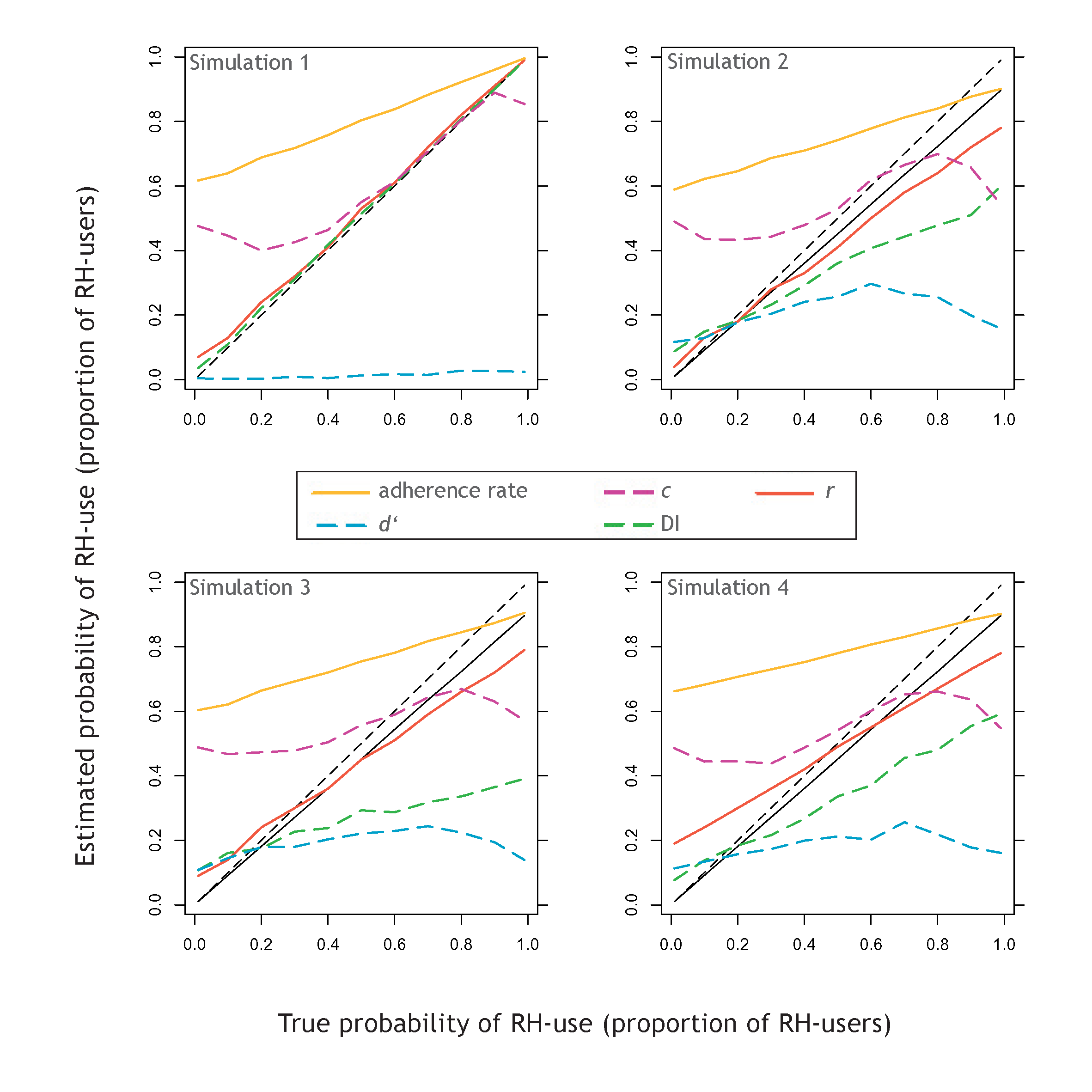
| Figure 2: Simulation results under optimal conditions and
typical cue validities (top left), adding strategy execution errors
(top right), adding extremely high recognition and low knowledge
validity (bottom left), and forcing the recognition and knowledge cue
patterns to correlate positively (bottom, right). The adherence rate
(yellow) and r parameter (red) are compared against the
overall probability of RH use (solid black line). The DI (dashed
green), d′ (dashed blue) and c
(dashed purple) are compared against the proportion of RH-users in each
sample (dashed black line). |
3.1 Simulation 1: optimal conditions and typical cue
validities
The first simulation was run implementing optimal conditions for
identification of RH-use versus non-use. First, in this simulation,
there was no strategy execution error; thus, the overall probability of
RH-use and the proportion of RH-users in the sample are equivalent.
Therefore, all measures can be compared against the same criterion,
viz. the true underlying proportion of RH-users in each data set.
Secondly, the random noise probabilities when drawing the cue patterns
were chosen to result in a mean recognition validity of .75 and mean
knowledge validity of .65 (thus mirroring typical data sets, Hilbig et
al., 2010); specifically, the individual probability of random noise
was drawn from a normal distribution with M = .10, SD
= .05, and M = .20, SD = .05 for the recognition and
the knowledge cue, respectively. In the following simulations 2 to 4
these constraints will be manipulated to assess the robustness of the
measures investigated.
The results of this first simulation are shown in the top left panel of
Figure 2 which plots the estimated probability of RH-use (proportion of
RH-users) against the true underlying proportion of users. Optimal
estimates would lie on the diagonal (dashed black line).
Table 1 additionally provides, for each measure, the mean absolute
deviation, sum of squared differences, and maximally observed deviation
from the true criterion across the eleven simulated data sets. As can
be seen, the adherences rate substantially and consistently
overestimated the probability of RH-use by up to .61 and with a mean
absolute deviation of .30. Thus, even under optimal conditions, the
adherence rate performed poorly and, as Figure 2 clearly demonstrates,
severely overestimated use of the RH.
Surprisingly, the d′ measure also performed
poorly, as it practically predicted no RH-use at all. As the severe
underestimation provided by this measure (see Figure 2) indicates, the
criterion of classifying only those decision makers as RH-user who
score d′ = 0 is too strict. This is especially
interesting in light of the very satisfying performance of the DI which
used the same classification criterion (DI = 0) and, as introduced
above, is almost tantamount to d′, except for
the lack of z-transformation. The DI, however, was almost perfectly
related to the true criterion (with a mean absolute deviation of .01),
and actually outperformed all other measures in the set (see Table 1).
The performance of c, by contrast, was relatively poor as
indicated by a maximally observed deviation of .47. Interestingly, for
true criterion values between .40 and .90, this measure performed very
well and comparable to the DI. However, especially in case of lower
true proportions of RH-users, c yielded severe overestimation
of RH-use. Worse yet, the proportion of estimated RH-users obtained
from c was not a monotonic function of the true underlying
proportion of RH-users (see Figure 2). So, conclusive interpretation of
differences in c as more versus less RH-use is not warranted
— even under optimal conditions.
Finally, the r parameter estimated with the r-model showed very
good performance (mean absolute deviation of .02) which was highly
comparable to the DI. Indeed, the very small differences between the
two should not be overemphasized. Rather, under the perfect conditions
and typical cue validities implemented in this simulation, both
measures provided very accurate estimation of RH-use or the proportion
of RH-users.
3.2 Simulation 2: Strategy execution error
The assumptions implemented in the above reported simulation are,
admittedly, not entirely realistic. Most importantly, simulated
participants’ strategy execution was perfect, that is,
no errors occurred. In real empirical data, however, it is unlikely
that this would hold (e.g., Glöckner, 2009; Rieskamp, 2008).
Therefore, in the next simulation, an individual error probability was
set for each participant, randomly drawn from a normal
distribution with M = .10 and SD = .05. On each
trial, after the choice had been determined, this choice was switched
with the probability of an error. As a consequence, even a true RH-user
would now, on some trials, choose the unrecognized object.
Note that under these conditions the true underlying proportion of
RH-users and the overall probability of RH-use are no longer the same.
Therefore, the adherence rate and the r parameter were
evaluated against the actually resulting overall probability of RH-use
(solid black line in Figure 2), whereas d′, c, and the DI
were again compared to the underlying proportion of RH-users (dashed
black line). Additionally, because the classification criterion of
d′ and the DI is unrealistic when strategy execution errors
must be expected, both were allowed a more lenient criterion. For the
DI, any simulated participant scoring within −.05 ≤ DI
≤ .05 was classified as a RH-user. While the DI has a
possible range from −1 to 1, d′ can practically take values
anywhere between −3 and 3. Thus, the classification criterion was
three times as large as for the DI, specifically −.15 ≤
d′ ≤ .15.4 The results of this simulation
are provided in Table 1 and displayed in the top right panel of Figure
2. As could be expected, most measures suffered from the addition of
strategy execution errors. However, they were affected differentially:
The adherence rate did not perform notably worse, but merely
maintained its consistent and severe overestimation of RH-use. The
d′ measure, though again performing worst of all, actually
improved. Obviously, this is due to the more lenient classification
criterion implemented. However, the estimated proportion of RH-users
derived from d′ was non-monotonically related to the
underlying true proportion (see Figure 2) which severely limits the
interpretability of this measure. In any case, d′ was
clearly outperformed by all other measures — even the simple
adherence rate.
All other measures were now negatively affected. Both c and the DI
performed notably worse, with estimates diverging from the true
proportion of RH-users by as much as .48 and .39, respectively. Under
the current conditions, the fit statistics provided only weak evidence
for the superiority of the DI over c. However, Figure 2 (top, right)
does indicate that c was again a non-monotonic function of the true
underlying proportion of RH-users. As is the case for d′,
this is a drawback which strongly limits interpretability of
c. While the DI also performed notably worse than under optimal
conditions, it did at least retain its monotonic relation to the true
to-be-estimated criterion.
The r parameter estimated from the r-model, too, no longer
performed optimally. Indeed, it now produced estimates diverging from
the true probability of RH-use by as much as .11. On the other hand,
the fit statistics unequivocally indicated that r was now the
best-performing measure in the set (see Table 1). Its mean absolute
deviation of .05 is less than a third of the according statistic for
the second-best measure, the DI.
3.3 Simulation 3: Extreme validities
So far, the cue validities implemented in the simulations were
intermediate in size and reflected the typically observed difference
between the recognition and knowledge validity. However, it may occur
that the recognition validity is much larger than the knowledge
validity and quite extreme in absolute terms (Hilbig & Richter, in
press). As a result, there will be much fewer cases in which the RH
actually yields a false prediction. This fact in turn should affect measures
placing particular emphasis on such cases (especially the DI). To
manipulate the cue validities, the random noise probabilities were
changed: For the recognition cue, there was no longer any random noise;
for the knowledge cue, the random noise probability was drawn from a
normal distribution with M = .25 and SD = .05.
Consequently, the mean recognition validity increased to .90, while the
mean knowledge validity dropped to .55. Otherwise this simulation was
exactly the same as the previous one (including strategy execution
errors).
The results are shown in the lower left panel of Figure 2 and fit
statistics are again found in Table 1. As could be expected, the
resulting decrease in performance was most obvious for the DI, which
now actually performed worse than the c measure in terms of fit
statistics. Clearly, the extremely large recognition validity led to
increasingly severe underestimation of the true underlying proportion
of RH-users by the DI. The performance of d′ and c, by
contrast, was not as strongly affected but merely remained generally
poor. Also, both were again non-linearly related to the underlying
criterion, thus hampering interpretability. On a more positive note,
the r parameter was not affected by the extreme
validities. In fact, it performed exactly as in the previous
simulation with a very satisfying mean absolute deviation of .05.
3.4 Simulation 4: Cue inter-correlation
In a final simulation, another potential caveat for strategy
classification other than extreme validities was sought. Specifically,
the recognition and knowledge cue patterns were now forced to correlate
positively (r ≥ .3). To implement this restriction, a naïve
method was used which simply computed the correlation of the two cue
patterns and redrew cue values if the condition of r ≥ .3 was
not fulfilled. However, as a consequence, the cue validities were also
affected. Therefore, the random noise probabilities were adjusted to
render the current simulation comparable to the first two: The
probabilities were drawn from normal distributions with M =
.30, SD = .05 and M = .05, SD = .05 for the
recognition and knowledge cue, respectively, resulting in a mean
recognition validity of .75 and mean knowledge validity of .64. This
simulation was thus exactly the same as Simulation 2 (including
strategy execution errors), apart from the addition of positive
cue-pattern correlations which will again render strategy
identification more difficult because less diagnostic cases occur when
cues are correlated (Glöckner, 2009). In other words, the knowledge
cue was substantially less likely to argue against a recognized object.
The results are depicted in the lower right panel of Figure 2
(see also Table 1). Whereas the performance of most measures only
worsened slightly compared to Simulation 2, the r parameter now showed
less satisfactory fit statistics. The effect of introducing cue-pattern
correlations on the r estimate is clearly visible by comparing the
upper and lower right panels of Figure 2: The r parameter now tended to
overestimate RH-use when the true underlying proportion of RH-users was
small. This is plausible given that the positive cue-pattern
correlation will increase the probability of a RH-non-user following
the recognition cue — simply because the knowledge cue is less likely
to argue against it. However, these findings notwithstanding, the
r parameter was still the best-performing measure in the set and its
mean absolute deviation of .08 can still be considered satisfactory.
3.5 Summary and discussion of simulation results
Several measures for assessing the probability of RH-use or,
alternatively, the proportion of RH-users in a sample were compared in
a set of simulations. As a starting point, optimal conditions for
strategy identification were implemented, namely no strategy execution
errors, typical cue validities, and independently drawn cue patterns.
The results of this simulation revealed that both the adherences rate
and Pachur and Hertwig’s (2006) d′ performed poorly. That is,
even assuming optimal conditions, these measures should not be applied
to assess RH-use. By contrast, c performed more acceptably in
terms of fit and especially for larger underlying proportions of
RH-users. However, at lower levels, c showed a varying
tendency to overestimate RH-use and, worse yet, was a non-monotonic
function of the to-be-estimated criterion which is a severe
drawback. Neither of these problems were apparent for the DI (Hilbig
& Pohl, 2008) which provided highly accurate estimates of the
proportion on RH-users in the simulated samples. Likewise, the
r parameter as estimated from the multinomial processing tree
model proposed by Hilbig, Erdfelder, and Pohl (2010) showed almost
perfect performance.
In the following simulations, the implemented constraints ensuring
optimal conditions for strategy identification were relaxed.
Specifically, strategy execution errors were introduced, extreme
validities were implemented, and positive cue-pattern correlations were
enforced. Overall, those measures originally performing well (DI and
r) did suffer from these obstacles. In particular, the DI
strongly underestimated higher proportions of RH-users in a sample when
an extremely large recognition validity (.90) and very low knowledge
validity (.55) were implemented. The r parameter, by contrast, provided
adequate estimates under these circumstances but performed less well
when positive cue-pattern correlations were enforced. On the whole,
however, the r parameter provided the best estimates of RH-use which
held even under conditions clearly hampering optimal strategy
classification.
4 Measure evaluation through empirical data
Simulations bear advantages and limitations. One of the latter is that
the behavior of actual decision makers can, at best, only be
approximated. In a second step, I thus sought to evaluate the different
measures of RH-use through empirical data. However, as outlined in the
introduction, the paradigm of natural recognition (without any control
over participants’ cue knowledge) cannot provide any
useful comparison against which to evaluate these measures. Instead, it
is much more informative to apply these measures to data in which the
cue patterns are known and RH-use can be assessed using the
strategy-classification method of Bröder and Schiffer (2003). The
combination of this method with diagnostic tasks yields vastly more
control and allows for more conclusive classification of participants
to strategies.
Specifically, the data of Glöckner and Bröder (in press) were analyzed
because the authors implemented a paradigm in which participants were
provided with additional information beyond recognition: Participants
were shown recognized and unrecognized US-cities and were additionally
given information about these, namely three additional cues. Based on
the artificially created cue patterns, participants’
choice data were analyzed with the Bröder/Schiffer-method. As
reported by Glöckner and Bröder (in press, Figure 1), a proportion of
up to 36.25% of their sample were accordingly classified as users of
non-compensatory strategies such as the RH.
The question then was how the measures of RH-use investigated herein
would perform as compared to the
Bröder/Schiffer-method. Importantly, all these measures ignore
information about the cue patters in specific trials. So, from
Glöckner and Bröder’s data, I kept only the three pieces of
information necessary for computing the measures of RH-use: (i) which
objects were compared on each trial, (ii) which objects participants
reported to recognize, and (iii) actual choices. For those measures
which afford some fixed criterion to classify participants as
RH-users, the following were used: A participant with a DI within the
95%-confidence-interval of zero (± .11) was classified as a
RH-user (cf. Hilbig & Pohl, 2008). The same criterion (±
.07) was used for d′. For c, participants with values
smaller than the upper bound of the 95%-confidence-interval of zero
(.11) were considered RH-users. The remaining measures, viz. the
adherence rate and the r parameter, again estimated the
overall probability of RH-use.
Results were mostly consistent with what might be expected from the
simulations reported above. The mean adherences rate in the sample was
.71 (SD = .14), thereby severely overestimating RH-use as
compared to the results of the Bröder/Schiffer-method. Also,
d’ showed the same strong underestimation which was already
visible in the simulations, proposing that only 6% of participants
were RH-users. Overall, c and the DI yielded more accurate
estimates, implying proportions of RH-users in the sample of .52 and
.59, respectively. Clearly, both performed better than the adherence
rate and d′, but neither provided an estimate which was
satisfyingly close to what was expected from the maximum-likelihood
strategy classification. Finally, the r-model (which fit the empirical
data well, G²(1) = .12, p = .74)
estimated the overall probability of RH-use to be r = .40
(SE = .01) which is close to the conclusion drawn from the
Bröder/Schiffer-method, namely that about 36% of participants were
most likely to have used the RH.
In sum, once more, the r-model provided the best estimate of RH-use —
though, unlike in the simulations, “best” here does not refer to the
known underlying truth but rather to the results obtained from a
well-established and widely-used method for strategy classification.
However, one may argue that this method need not uncover the actual
judgment processes — especially if only choices are considered
(Glöckner, 2009). Therefore, from the current analysis, it might be
more adequate to conclude that the r-model provides the estimate of
RH-use closest to what is implied by Bröder and Schiffer’s (2003)
maximum-likelihood strategy-classification method (and no
more). Importantly, though, the r-model achieves this without
considering any information about cue patterns in the different
trials.
| Table 2: Results concerning desirable criteria for measurement
tools of RH-use. |
| | Measures |
| | AR | d’ | c | DI | r |
Directly interpretable estimate of RH-use | yes | no | no | no | yes |
Adequate estimate of RH-use (under optimal conditions) | no | no | no | yes | yes |
Adequately robust (under non-optimal conditions) | * | * | * | yes** | yes*** |
Estimate monotonically related to RH-use | yes | no | no | yes | yes |
Parallel results to maximum-likelihood strategy classification in
empirical data | no | no | yes | no | yes |
Goodness-of-fit tests | no | no | no | no | yes |
| * It makes little sense to interpret the robustness
of measures which performed poorly even under optimal conditions. |
| ** The DI is least robust if the recognition validity is extremely high
and much larger than the knowledge validity. |
| *** The r-estimate is
least robust if recognition and knowledge cue patterns correlate
positively. |
5 Discussion
Concerning the recognition heuristic (RH; Goldstein & Gigerenzer,
2002), most of the recent investigations have concluded that it neither
represents a general description of comparative judgments nor appears
to be refutable altogether (Hilbig, in press) — very much like the
take-the-best heuristic (Bröder & Newell, 2008). Consequently, it is
an important quest to uncover the conditions and individual differences
which foster or hamper application of simple one-cue strategies, such
as the RH. However, mutual progress in this domain would necessitate
some consensus as to the paradigms and measures appropriate for
investigating use of this strategy. So far, there has been some work
concerning suitable paradigms and it is my impression that using
naturally recognized objects without teaching (or providing) any
further cue knowledge or information has emerged as one preferred
method (Pachur et al., 2008) — especially given that the potential
dangers of participants possessing criterion knowledge need not be too
severe (Hilbig, Pohl, & Bröder, 2009).
However, such a paradigm in which there is no control over
participants’ knowledge beyond recognition renders measurement of
RH-use very difficult. Clearly, choices in line with a single-cue
strategy provide little information about its actual use, if other
cues (the values of which are unknown) may imply the same choice
(Bröder & Eichler, 2006; Bröder & Schiffer, 2003; Hilbig, 2008b,
in press). In this article, I have therefore considered different
measures and evaluated them with respect to their ability of
uncovering true use of the RH. Specifically, apart from the adherence
rate (proportion of choices in line with the RH), Pachur and Hertwig’s
(2006) d′ and c (Pachur et al., 2009), the
discrimination index (DI; Hilbig & Pohl, 2008), and the parameter
r from the r-model (Hilbig et al., 2010) were compared.
Table 2 summarizes the main results with respect to several desirable
criteria. Firstly, only the adherence rate and r-model provide a
directly interpretable estimate of RH-use; d′, c and
DI, by contrast, necessitate further assumptions as to the values
RH-users would show (as a necessary but not sufficient condition, cf.
Hilbig & Pohl, 2008). Secondly, DI and r provide adequate
estimates of RH-use under optimal conditions, whereas c, the
adherence rate, and d′ perform less convincingly: While the
adherences rate consistently and severely overestimated RH-use, the
exact opposite was the case for d′. Furthermore, d′
and c were mostly non-monotonically related to the true
proportion of RH-users which hampers the interpretability of
differences in these measures. Overall, only r was
satisfactorily robust against less optimal conditions for strategy
identification — though situations bearing a substantial positive
correlation between recognition and knowledge cue patterns do pose
difficulties for this measure, too.
Additionally, I asked which measures would produce results similar to
choice-based maximum-likelihood strategy-classification (Bröder &
Schiffer, 2003; Glöckner, 2009) in Glöckner and Bröder’s (in press)
empirical data. The most comparable estimates were provided by c
and, even more so, the r parameter. Finally, as an additional
benefit, the r-model allows for goodness-of-fit tests and comprises
many of the other advantageous features of multinomial processing tree
models (Erdfelder et al., 2009) — including, for example, model
comparisons with respect to goodness-of-fit and complexity
(Myung, 2000). Also, in light of recently developed free and
platform-independent software for analysis of multinomial models
(Moshagen, 2010), the r-model is no more difficult to apply than any
of the other measures.
In sum, for those studying comparative judgments between naturally
recognized objects (without teaching or providing further cues), the
r-model will yield the best measure of RH-use currently available.
However, there are also situations in which this measurement tool will
not be helpful and I consider it important to point to these cases:
Firstly, the r-model cannot be applied to preferential choice, that is,
situations in which there is no conclusive criterion which choice
option represents a correct versus false judgment. In fact, this
limitation applies to all measures discussed herein except for the
adherence rate. Secondly, the r-model is designed for exhaustive
paired-comparisons as it affords cases in which both objects are
recognized and cases in which only one is recognized. At
least, a representative sample of each of these sets of cases is
necessary. This limitation does not hold for any of the other measures,
each of which can be applied to only those cases in which exactly one
object is recognized. On the other hand, I am aware of few empirical
investigations which actually were limited to such cases.
Beyond some recommendations for measuring RH-use, what methodological
conclusions can be drawn? As the extremely poor performance of the
adherence rate (which is the measure most often applied so far)
indicates, more careful consideration of our measurement tools seems
advisable. Precisely formulated process models of judgment and
decision making deserve precise (and process-pure) measures. So long
as measurement is vague, exact description on the theoretical level
will not avail us. With good reason, Gigerenzer and colleagues have
called for precise theories (Gigerenzer, 1996, 2009; Gigerenzer,
Krauss, & Vitouch, 2004). However, it does not suffice — though it
is necessary — to build precise theories. If we do not add a call for
using the most precise measurement tools available, we may too often
fall prey to premature conclusions. For the recognition heuristic
theory, I hope to have provided some insight which measures are more
or less likely to enhance our understanding.
References
Batchelder, W. H., & Riefer, D. M. (1999). Theoretical and empirical
review of multinomial process tree modeling. Psychonomic
Bulletin & Review, 6, 57–86.
Bröder, A. (in press). The quest for Take The Best: Insights and
outlooks from experimental research. In P. Todd, G. Gigerenzer, & the
ABC Research Group (Eds.), Ecological rationality: Intelligence
in the world. New York: Oxford University Press.
Bröder, A., & Eichler, A. (2006). The use of recognition information
and additional cues in inferences from memory. Acta
Psychologica, 121, 275–284.
Bröder, A., & Newell, B. R. (2008). Challenging some common beliefs:
Empirical work within the adaptive toolbox metaphor. Judgment
and Decision Making, 3, 205–214.
Bröder, A., & Schiffer, S. (2003). Bayesian strategy assessment in
multi-attribute decision making. Journal of Behavioral Decision
Making, 16, 193–213.
Bröder, A., & Schiffer, S. (2006). Adaptive flexibility and
maladaptive routines in selecting fast and frugal decision strategies.
Journal of Experimental Psychology: Learning, Memory, and
Cognition, 32, 904–918.
Erdfelder, E., Auer, T.-S., Hilbig, B. E., Aßfalg, A., Moshagen, M.,
& Nadarevic, L. (2009). Multinomial processing tree models: A review
of the literature. Zeitschrift für Psychologie - Journal of
Psychology, 217, 108–124.
Erdfelder, E., Küpper-Tetzel, C. E., & Mattern, S. (2010).
Threshold models of recognition and the recognition heuristic.
Manuscript submitted for publication.
Gigerenzer, G. (1996). On narrow norms and vague heuristics: A reply to
Kahneman and Tversky. Psychological Review, 103, 592–596.
Gigerenzer, G. (2009). Surrogates for theory. APS Observer, 22,
21–23.
Gigerenzer, G., Krauss, S., & Vitouch, O. (2004). The Null Ritual: What
you always wanted to know about significance testing but were afraid to
ask. In D. Kaplan (Eds.), The Sage handbook of quantitative
methodology for the social sciences (pp. 391–408). Thousand Oaks:
Sage Publications.
Glöckner, A. (2009). Investigating intuitive and deliberate processes
statistically: The multiple-measure maximum likelihood strategy
classification method. Judgment and Decision Making, 4,
186–199.
Glöckner, A., & Betsch, T. (2008). Multiple-reason decision making
based on automatic processing. Journal of Experimental
Psychology: Learning, Memory, & Cognition, 34, 1055–1075.
Glöckner, A., & Bröder, A. (in press). Processing of recognition
information and additional cues: A model-based analysis of choice,
confidence, and response time. Judgment and Decision Making
Goldstein, D. G., & Gigerenzer, G. (1999). The recognition heuristic:
How ignorance makes us smart. In G. Gigerenzer, P.M. Todd, & The ABC
Research Group (Eds.), Simple heuristics that make us smart
(pp. 37–58). New York: Oxford University Press.
Goldstein, D. G., & Gigerenzer, G. (2002). Models of ecological
rationality: The recognition heuristic. Psychological Review,
109, 75–90.
Hilbig, B. E. (2008a). Individual differences in fast-and-frugal
decision making: Neuroticism and the recognition heuristic.
Journal of Research in Personality, 42, 1641–1645.
Hilbig, B. E. (2008b). One-reason decision making in risky choice? A
closer look at the priority heuristic. Judgment and Decision
Making, 3, 457–462.
Hilbig, B. E. (in press). Reconsidering “evidence” for fast and
frugal heuristics. Psychonomic Bulletin & Review.
Hilbig, B. E., Scholl, S., & Pohl, R. F. (2010). Think or blink – is
the recognition heuristic an “intuitive” strategy? Judgment
and Decision Making, 5, 300–309.
Hilbig, B. E., Erdfelder, E., & Pohl, R. F. (2010). One-reason
decision-making unveiled: A measurement model of the recognition
heuristic. Journal of Experimental Psychology: Learning,
Memory, & Cognition, 36, 123–134.
Hilbig, B. E., & Pohl, R. F. (2008). Recognizing users of the
recognition heuristic. Experimental Psychology, 55, 394–401.
Hilbig, B. E., & Pohl, R. F. (2009). Ignorance- versus evidence-based
decision making: A decision time analysis of the recognition heuristic.
Journal of Experimental Psychology: Learning, Memory, and
Cognition, 35, 1296–1305.
Hilbig, B. E., Pohl, R. F., & Bröder, A. (2009). Criterion knowledge:
A moderator of using the recognition heuristic? Journal of
Behavioral Decision Making, 22, 510–522.
Hilbig, B. E., & Richter, T. (in press). Homo heuristicus outnumbered:
Comment on Gigerenzer and Brighton (2009). Topics in Cognitive
Science.
Jekel, M., Nicklisch, A., & Glöckner, A. (2010). Implementation of
the Multiple-Measure Maximum Likelihood strategy classification method
in R: addendum to Glöckner (2009) and practical guide for
application. Judgment and Decision Making, 5, 54–63.
Macmillan, N. A., & Creelman, C. D. (2005). Detection theory: A
user’s guide (2nd ed.). NJ, US: Lawrence Erlbaum
Associates Publishers.
Marewski, J. N., Gaissmaier, W., Schooler, L. J., Goldstein, D. G., &
Gigerenzer, G. (2010). From recognition to decisions: Extending and
testing recognition-based models for multi-alternative inference.
Psychonomic Bulletin & Review, 17, 287–309.
Moshagen, M. (2010). multiTree: A computer program for the analysis of
multinomial processing tree models. Behavior Research Methods,
42, 42–54.
Myung, I. J. (2000). The importance of complexity in model selection.
Journal of Mathematical Psychology, 44, 190–204.
Newell, B. R., & Fernandez, D. (2006). On the binary quality of
recognition and the inconsequentially of further knowledge: Two
critical tests of the recognition heuristic. Journal of
Behavioral Decision Making, 19, 333–346.
Newell, B. R., & Shanks, D. R. (2004). On the role of recognition in
decision making. Journal of Experimental Psychology: Learning,
Memory, and Cognition, 30, 923–935.
Oppenheimer, D. M. (2003). Not so fast! (and not so frugal!): Rethinking
the recognition heuristic. Cognition, 90, B1-B9.
Pachur, T., Bröder, A., & Marewski, J. (2008). The recognition
heuristic in memory-based inference: Is recognition a non-compensatory
cue? Journal of Behavioral Decision Making, 21, 183–210.
Pachur, T., & Hertwig, R. (2006). On the psychology of the recognition
heuristic: Retrieval primacy as a key determinant of its use.
Journal of Experimental Psychology: Learning, Memory, and
Cognition, 32, 983–1002.
Pachur, T., Mata, R., & Schooler, L. J. (2009). Cognitive aging and the
adaptive use of recognition in decision making. Psychology & Aging, 24, 901–915.
Pohl, R. F. (2006). Empirical tests of the recognition heuristic.
Journal of Behavioral Decision Making, 19, 251–271.
Richter, T., & Späth, P. (2006). Recognition is used as one cue among
others in judgment and decision making. Journal of Experimental
Psychology: Learning, Memory, and Cognition, 32, 150–162.
Rieskamp, J. (2008). The probabilistic nature of preferential choice.
Journal of Experimental Psychology: Learning, Memory, and
Cognition, 34, 1446–1465.
Schooler, L. J., & Hertwig, R. (2005). How forgetting aids heuristic
inference. Psychological Review, 112, 610–628.
This document was translated from LATEX by
HEVEA.