Judgment and Decision Making, vol. 5, no. 4, July 2010, pp. 244-257
The less-is-more effect: Predictions and testsKonstantinos V. Katsikopoulos* |
In inductive inference, a strong prediction is the less-is-more effect: Less information can lead to more accuracy. For the task of inferring which one of two objects has a higher value on a numerical criterion, there exist necessary and sufficient conditions under which the effect is predicted, assuming that recognition memory is perfect. Based on a simple model of imperfect recognition memory, I derive a more general characterization of the less-is-more effect, which shows the important role of the probabilities of hits and false alarms for predicting the effect. From this characterization, it follows that the less-is-more effect can be predicted even if heuristics (enabled when little information is available) have relatively low accuracy; this result contradicts current explanations of the effect. A new effect, the below-chance less-is-more effect, is also predicted. Even though the less-is-more effect is predicted to occur frequently, its average magnitude is predicted to be small, as has been found empirically. Finally, I show that current empirical tests of less-is-more-effect predictions have methodological problems and propose a new method. I conclude by examining the assumptions of the imperfect-recognition-memory model used here and of other models in the literature, and by speculating about future research.
Keywords: less-is-more effect, recognition heuristic, recognition memory.
In psychology’s quest for general laws, the effort-accuracy tradeoff (Garrett, 1922; Hick, 1952) is a top candidate: The claim is that a person cannot put less effort in a task and increase accuracy. Because it is widely accepted, the tradeoff provides an opportunity for theory development. If a theory implies that the effort-accuracy tradeoff can be violated, this is a strong prediction. By strong prediction of a theory I mean a prediction that does not follow from most competing theories (see Trafimow, 2003). A strong prediction provides for informative tests. It is unlikely that the data will confirm the prediction, but if they do, support for the theory will increase greatly. For example, Busemeyer (1993) provided support for decision field theory by showing that it is consistent with violations of the speed-accuracy tradeoff.
The speed-accuracy tradeoff is one instantiation of the effort-accuracy tradeoff in which the effort a person puts into performing a task is measured by the time she uses. Effort can also be measured by the amount of other resources that are expended, such as information or computation. In this paper, I consider violations of the tradeoff between information and accuracy. This violation is particularly interesting because it invites us to sometimes throw away information. This invitation flies in the face of epistemic responsibility, a maxim cherished by philosophers and practitioners of science (Bishop, 2000). Some violations of the information-accuracy tradeoff, where information refers to recognition, have been predicted and observed in tasks of inductive inference, and are collectively referred to as the less-is-more effect (Gigerenzer, Todd, & the ABC research group, 1999).
Here, I make two kinds of contributions to the study of the less-is-more effect: to the theoretical predictions of the effect, and to the empirical tests of the predictions. Specifically, in the next section, I define the inference task and the less-is-more effect, and present Goldstein and Gigerenzer’s (2002) characterization of the less-is-more effect for the case of perfect memory. In Section 3, for imperfect memory, I derive a more general characterization of the conditions under which the less-is-more effect is predicted. The predictions are illustrated numerically with parameter estimates from the recognition memory literature. Furthermore, I discuss implications for theoretical explanations of the effect. A new type of less-is-more effect is also predicted. In the next section, I discuss methodological issues in empirically testing less-is-more effect predictions, and present a method for doing so by using data from recognition experiments. In Section 5, I conclude by examining the assumptions of the imperfect-memory model used here and of other models in the literature, and by speculating about future research.
I first define the inference task: There exist N objects that are ranked, without ties, according to a numerical criterion. For example, the objects may be cities and the criterion may be population. A pair of objects is randomly sampled and the task is to infer which object has the higher criterion value. When recognition memory is perfect, a person’s information is modeled by the number of objects she recognizes, n, where 0 ≤ n ≤ N. The person’s accuracy is the probability of a correct inference and it is a function of her information, Pr(n). I next define the less-is-more effect.
When recognition memory is perfect, the
less-is-more effect occurs if and only if there exist n1 and n2
such that n1 < n2 and Pr(n1) > Pr(n2).
The less-is-more effect may at first appear to be impossible: Of
course, whatever processing can be done with less information
(recognizing n1 objects), could also be done when adding
information (recognizing the same n1 objects and an extra n2 −
n1 objects); so, how can less information lead to more accuracy? The
catch is that different amounts of information may lead to different
processing. For example, when the population of two cities is
compared, recognizing the name of one of the two cities enables the
recognition heuristic (Goldstein & Gigerenzer, 2002):
“If one object is recognized and the other object is not, the
recognized object is inferred to have the higher criterion value.”
The recognition heuristic cannot be used when both objects are
recognized so that some other inference rule has to be used, such as
a linear rule with unit weights (Dawes & Corrigan, 1974). The
processing done with less information may be more accurate than
the processing done with more information. For example, the
recognition heuristic uses one cue (recognition) and there are
conditions under which using one cue is more accurate than summing
many cues (Hogarth & Karelaia, 2005; Katsikopoulos & Martignon,
2006; this point has also been made specifically for the recognition
cue by Davis-Stober, Dana, & Budescu, 2010).
To test empirically the occurrence of the less-is-more effect, one can compare the accuracy of (i) two agents (individuals or groups) who recognize different amounts of objects out of the same set (e.g., American cities), or (ii) the same agent who recognizes different amounts of objects in two different sets (e.g., American and German cities).
Pachur (in press) reviewed a number of studies and concluded that there is some evidence for the less-is-more effect in some experiments, but not in others. I agree with this conclusion: Goldstein and Gigerenzer (2002) had about a dozen American and German students infer which one of San Diego or San Antonio is more populous, and found that the Germans were more accurate (1.0 vs. .67). They also found that 52 American students were equally accurate (.71) in making 100 population comparisons of German, or American cities. Reimer and Katsikopoulos (2004) had three-member groups of German students perform 105 population comparisons of American cities. Out of seven pairs of groups, the groups who recognized fewer cities were more accurate in five cases, by .04 on the average. Pohl (2006) had 60 German students compare the populations of 11 German, 11 Italian, and 11 Belgian cities. The students recognized more German than Italian cities and more Italian than Belgian cities, and their accuracies had the same order: .78 for German, .76 for Italian, and .75 for Belgian cities. Pachur and Biele (2007) asked laypeople and soccer experts to forecast the winners of matches in the 2004 European national-teams soccer tournament. In 16 matches, experts were more accurate than laypeople (.77 vs. .65). The correlation between the accuracy of 79 laypeople and the number of teams they recognized was positive (.34).
I believe that all of these tests of less-is-more-effect predictions have methodological problems and I will make this point and suggest a new method in Section 4.
Goldstein and Gigerenzer (2002) derived an equation for Pr(n) based on a model of how a person makes inferences, which I now describe. The first assumption of the perfect-memory model is the following:
The person recognizes all objects she has
experienced, and does not recognize any object she has not
experienced.
It is easy to criticize this assumption as it is known that
recognition memory is not perfect (Shepard, 1967). Pleskac (2007) and
Smithson (2010) proposed models of imperfect recognition memory,
and I will discuss them together with a new model, in Section 3.
The following three assumptions specify the inference rules used for the different amounts of recognition information that may be available:
If the person does not recognize any of the objects in the pair, she uses guessing to infer which object has the higher criterion value.
If the person recognizes one object, she uses the recognition heuristic.
If the person recognizes both objects, she
uses an inference rule other than guessing or the recognition
heuristic-this family of rules is labeled as knowledge.
Based on Assumptions (2)–(4), if the person recognizes n of the
N objects, she uses guessing, recognition heuristic, and knowledge
with the following respective probabilities:
|
The last assumption of the perfect-memory model is the following:
The accuracy of the recognition
heuristic,α, and the accuracy of knowledge, β, are
constant across n (and α, β > 1/2 ).
Smithson (2010) pointed out that Assumption 5 could be potentially
violated, and constructed plausible examples where this is the
case.1 Pachur and Biele (2007) reported that the
correlation between α and n was .19 and the correlation
between β and n was .22. Across ten experiments, Pachur (in
press) reported that the average of the absolute value of the
correlation between α and n was .27 and the average of the
absolute value of the correlation between β and n was .18. In
Section 4, I will argue that the estimates of α and β
used in these studies are incorrect, and the reported correlations
should be interpreted with caution.
From Assumption 5 and Equation (1), it follows that the accuracy of a person who recognizes n objects is given as follows:
| Pr(n) = g(n)(1/2) + r(n)α + k(n)β (2) |
Take N =100. If α = .8 and β =
.6, then Pr(50) = .68 and Pr(100) = .6, and a less-is-more effect
is predicted. If α = .8 and β = .8, then Pr(50) =
.73 and Pr(100) = .8, and more generally Pr(n1) < Pr(n2)
for all n1 < n2, and the effect is not predicted.
It is straightforward to study Equation (2) and derive the following
characterization of the less-is-more effect (Goldstein & Gigerenzer,
2002, p. 79):
For the perfect-memory model, the less-is-more effect is predicted if and only if α > β .2
More specifically, it holds that if α > β , there exists n* such that Pr(n*) > Pr(N): There is a person with an intermediate amount of information who is more accurate than the person with all information. And, if α ≤ β , then Pr(N) ≥ Pr(n) for all n < N, meaning that the person with all information makes the most accurate inferences.
The inference task is the same with that of Section 2: There exist N objects that are ranked, without ties, according to a numerical criterion; for example, the objects may be cities and the criterion may be population. A pair of objects is randomly sampled and the person has to infer which object has the higher criterion value. The person’s information is modeled by the number of objects she has experienced, ne, where 0 ≤ ne ≤ N. The person’s accuracy is the probability of a correct inference and it is a function of her information, Pr(ne). We have the following definition of the less-is-more effect.
When recognition memory is imperfect, the
less-is-more effect occurs if and only if there exist ne,1 and
ne,2 such that ne,1 < ne,2 and Pr(ne,1) >
Pr(ne,2).
I next propose a simple model of how people make inferences when
recognition memory is imperfect.
In this model, an experienced object that is recognized is called a hit; an experienced object that is not recognized is called a miss; a non-experienced object that is recognized is called a false alarm; and, a non-experienced object that is not recognized is called a correct rejection. A main assumption of my imperfect-memory model is the following:
Each experienced object has probability h
of being a hit, and each non-experienced object has probability f of
being a false alarm.
Assumption 1 of the perfect-memory model can be obtained from
Assumption 6 by setting h = 1 and f = 0. The differences between
the other assumptions of the imperfect- and perfect-memory models are
due to the fact that the role played by the recognition cue when
memory is perfect is played by the experience cue when memory is
imperfect. A person with imperfect memory cannot use the experience
cue (they have access only to the recognition cue), but let us still
define the experience heuristic:
“If one object is experienced and the other object is not, the
experienced object is inferred to have the higher criterion value.”
The experience heuristic is a convenient device for analyzing the
less-is-more effect. The following is assumed:
The accuracy of the experience heuristic,
A, and the accuracy of knowledge when both objects are experienced,
B, are constant across ne (and A, B > 1/2).
Assumption 7 generalizes Assumption 5 of the perfect-memory model because when memory is perfect it holds that A = α and B = β .
Now I specify the processing used for the different amounts of experience information that may be available. There are three types of pairs of objects that can be sampled, according to whether the number of experienced objects in the pair equals zero, one, or two. As in (1), these types occur with respective probabilities g(ne), r(ne), and k(ne). As Pleskac (2007) pointed out, accuracy depends not only on which of guessing, experience heuristic, or experience-based knowledge is used, but also on if each object in the pair is a hit, miss, false alarm, or correct rejection.
For example, assume that object 1 is experienced and object 2 is not experienced. There are four possibilities: (i) object 1 is a hit and object 2 is a correct rejection, (ii) object 1 is a hit and object 2 is a false alarm, (iii) object 1 is a miss and object 2 is a correct rejection, and (iv) object 1 is a miss and object 2 is a false alarm. In (i), the agent uses the recognition heuristic to make an inference because she recognizes only object 1. Because in this case the recognition and experience cues have the same value on both objects, it is as if the agent used the experience heuristic, and her accuracy equals A3.
Similarly, Pleskac (2007, p. 384-385) showed that accuracy equals 1 − A in (iv), 1/2 in (iii), and zA + (1 − z)(1/2) in (ii) (z is the probability that an experienced object has at least one positive value on a cue other than experience). Similarly, when the agent has experienced both objects, it can be shown that accuracy equals B if both objects are hits and 1/2 otherwise. When none of the two objects is experienced, it can be shown that accuracy always equals 1/2.
Pleskac interpreted h as the proportion of experienced objects that are recognized and f as the proportion of non-experienced objects that are recognized, and did not derive a simple equation for Pr(ne). When h and f are interpreted as probabilities, it is straightforward to do so according to the logic above, as follows:
Rewriting this, we get the main equation of the imperfect-memory model:
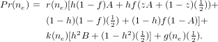
| Pr(ne) = g(ne)(1/2) + r(ne)αe + k(ne)βe, (3) |
where αe = (h − f + hfz)A +(1 − h + f − hfz)(1/2), and βe = h2B + (1 − h2)(1/2).
Equation (3) says that the inference task with imperfect recognition memory can be viewed as an inference task with perfect recognition memory where (i) the accuracy of the recognition heuristic αe equals a linear combination of the accuracy of the experience heuristic A and 1/2, and (ii) the accuracy of recognition-based knowledge βe equals a linear combination of the accuracy of experience-based knowledge B and 1/2. It holds that αe and βe are well defined in the sense that they lie between 0 and 1.
Take N =100. If A = .8, B = .8, h = .64, f = .02, and z = .5, then Pr(70) = .64 and Pr(100) = .62, and a less-is-more effect is predicted.
More generally, Figure 1 depicts graphically the conditions under
which the less-is-more effect is predicted, and Result 2 states and
proves this characterization.
Figure 1: The conditions under which the less-is-more effect is and is not predicted for the imperfect-memory model (A is the accuracy of the experience heuristic, B is the accuracy of experience-based knowledge, h is the probability of a hit, f is the probability of a false alarm, z is the probability that an experienced object has at least one positive value on a cue other than experience). For simplicity, the figure was drawn assuming that Kh/(1 − hz) > 0 and h/(1 − hz) < 1, but this is not necessarily the case. 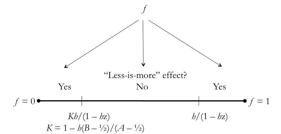
For the imperfect-memory model, the less-is-more effect is predicted if and only if either (i) f < Kh/(1 − hz), where K = 1 − h(B − 1/2)/(A − 1/2), or (ii) f > h/(1 − hz).
Note that if h − f + hfz > 0, (3) implies αe > 1/2. Also, note that it always holds that βe > 1/2.
Assume h − f + hfz > 0. Result 1 applies and the less-is-more effect is predicted if and only if αe > β e. The condition αe > β e can be rewritten as f < Kh/(1 − hz), where K = 1 − h(B − 1/2)/(A − 1/2). The condition h − f + hfz > 0 is equivalent to f < h/(1 − hz), which, because K < 1, is weaker than f < Kh/(1 − hz). Thus, if f < Kh/(1 − hz), the less-is-more effect is predicted.
The above reasoning also implies that if Kh/(1 − hz) ≤ f < h/(1 − hz), the less-is-more effect is not predicted. Also, if f = h/(1 − hz), then αe = 0, and the effect is not predicted.
Assume f > h/(1 − hz). Then, it holds that αe < 1/2 and Result 1 does not apply. The second derivative of Pr(ne) equals (1 − 2αe) + 2(βe − αe), which is strictly greater than zero because αe < 1/2 and αe < βe. Thus, Pr(ne) is convex, and a less-is-more effect is predicted.
Result 2 generalizes Result 1: For a perfect memory, it holds that h = 1, f = 0, A = α, and B = β . For h = 1 and f = 0, condition (ii) is always violated. From h = 1 and f = 0, condition (i) reduces to K > 0, which, because h = 1, is equivalent to A > B, or α > β .
Consistently with Result 2, if A = .8, B = .8, h = .64, f = .02, and z = .5, condition (i) is satisfied: f = .02 < .34 = Kh/(1 − hz), and a less-is-more effect is predicted. If A = .8, B = .8, h = .64, f = .64, and z = .5, then conditions (i) and (ii) in Result 2 are violated and a less-is-more effect is not predicted. If A = .8, B = .8, h = .37, f = .64, and z = .5, then condition (ii) in Result 2 is satisfied: f = .64 > .45 = h/(1 − hz), and a less-is-more effect is predicted; for example, Pr(0) = .5 > .48 = Pr(30). In paragraph 3.3, I discuss the meaning of this example in more detail. But first I differentiate between the two types of less-is-more effects in Result 2.
Table 1: The frequency, average prevalence, and average magnitude of the full-experience and below-chance less-is-more effects (see text for definitions), for the imperfect-memory model (varying A and B from .55 to 1 in increments of .05, and h, f, and z from .05 to .95 in increments of .05; and N = 100), and for the perfect-memory model (h = 1 and f = 0).
Frequency Frequency Avg. Prev. Avg. Prev. Avg. Mag. Avg. Mag. (Full Exp.) (B.Chance) (Full Exp.) (B.Chance) (Full Exp.) (B.Chance) Imperfect memory 29% 37% 23% 36% .01 .01 Perfect memory 50% 0% 23% 0% .02 .00
The predicted less-is-more effect is qualitatively different in each one of the two conditions in Result 2. If (i) is satisfied, Pr(ne) has a maximum and there exists a ne* such that Pr(ne*) > Pr(N), whereas if (ii) is satisfied, Pr(ne) has a minimum and there exists a ne* such that Pr(0) > Pr(ne*)4. In other words, in (i), there is a person with an intermediate amount of experience who is more accurate than the person with all experience, and in (ii), there is a person with no experience who is more accurate than a person with an intermediate amount of experience. I call the former a full-experience less-is-more effect and the latter a below-chance less-is-more-effect. The effects studied in the literature so far were of the full-experience (or full-recognition) type, interpreted as saying that there are beneficial degrees of ignorance (Schooler & Hertwig, 2005). The below-chance effect says that there could be a benefit in complete ignorance.
Result 2 tells us that the less-is-more effect is predicted, but not its magnitude. To get a first sense of this, I ran a computer simulation varying A and B from .55 to 1 in increments of .05, and h, f, and z from .05 to .95 in increments of .05 (and N = 100). There were 102 203 = 800,000 combinations of parameter values. For each combination, I checked whether the less-is-more effect was predicted, and, if yes, of which type. The frequency of a less-is-more effect type equals the proportion of parameter combinations for which it is predicted. For the combinations where an effect is predicted, two additional indexes were calculated.
The prevalence of a less-is-more effect equals the proportion of pairs (ne,1, ne,2) such that 0 ≤ ne,1 < ne,2 ≤ N and Pr(ne,1) > Pr(ne,2) (Reimer & Katsikopoulos, 2004). I report the average, across all parameter combinations, prevalence of the two less-is-more-effect types.
The magnitude of a less-is-more effect equals the average value of Pr(ne,1) − Pr(ne,2) across all pairs (ne,1, ne,2) such that 0 ≤ ne,1 < ne,2 ≤ N and Pr(ne,1) > Pr(ne,2). I report the average, across all parameter combinations, magnitude of the two less-is-more-effect types.
The simulation was run for both imperfect- and perfect-memory (where h = 1 and f = 0) models. The results are provided in Table 1. Before I discuss the results, I emphasize that the simulation assumes that all combinations of parameters are equally likely. This assumption is unlikely to be true, and is made because of the absence of knowledge about which parameter combinations are more likely than others.
The first result of the simulation is that the imperfect-memory model predicts a less-is-more effect often, abo3ut two-thirds of the time, 29% for the full-experience effect plus 37% for the below-chance effect. The perfect-memory model cannot predict a below-chance effect, and it predicts a lower frequency of the less-is-more effect (50%) than the imperfect-memory model. The second result is that, according to the imperfect-memory model, the below-chance effect is predicted to have higher average prevalence than the full-experience effect. Note also that the distribution of the prevalence of the below-chance effect is skewed: almost 50% of the prevalence values are higher than 45% (the prevalence distribution was close to uniform for the full-experience effect). The third result of the simulation is that the average magnitude of both less-is-more-effect types is small (.01 or .02); for example, in the imperfect-memory model, only about 5% of the predicted less-is-more effects have a magnitude higher than .05.5 This result is consistent with conclusions from empirical research (Pohl, 2006; Pachur & Biele, 2007; Pachur, in press). I would like to emphasize, however, that even small differences in accuracy could be important in the “real world”, as, for example, in business contexts.
In the predictions of the less-is-more effect in Example 2, we had A = B. This seems curious because a necessary and sufficient condition for predicting the effect when memory is perfect is α > β (see Result 1 and Example 1). In fact, Pleskac (2007) has argued that the condition A > B is necessary for the less-is-more effect when memory is imperfect.
The conditions α > β or A > B express that a heuristic (recognition or experience), is more accurate than the knowledge used when more information is available. If α > β or A > B, the less-is-more effect can be explained as follows: “Less information can make more likely the use of a heuristic, which is more accurate than knowledge.” This is an explanation commonly, albeit implicitly, proposed for the effect (e.g., Hertwig & Todd, 2003, Theses 2 & 3), and I call it the accurate-heuristics explanation.
Result 2 speaks against the accurate-heuristics explanation because it shows that A > B is neither necessary nor sufficient for predicting the less-is-more effect. The condition for the full-experience effect, f < Kh/(1 − hz), can be interpreted as indicating a small f and a medium h, where f and h can compensate for A ≤ B.6 The condition for the below-chance effect, f > h/(1 − hz), is independent of A and B, and can be interpreted as indicating a large f and a small h7 (simulations showed that z has a minor influence on both conditions).
In sum, Result 2 shows that it is the imperfections of memory (probabilities of misses and false alarms) that seem to drive the less-is-more effect, rather than whether the enabled heuristic (the experience heuristic) is relatively accurate or not.
I illustrate the evidence against the accurate-heuristics explanation by using parameter values from the recognition memory literature. Jacoby, Woloshyn, and Kelley (1989) provide estimates for h and f for the recognition of names.8 In each of two experiments, a condition of full attention and a condition of divided attention were run. In the divided-attention condition, participants were distracted by having to listen long strings of numbers and identify target sequences. In the full-attention condition, the average value of h was (.65 + .63)/2 = .64, and I used this value as an estimate of a high probability of a hit. In the divided-attention condition, the average h was (.43 + .30)/2 =.37, and this is my estimate of a low hit probability.
As an estimate of a low probability of a false alarm, I used the average value of f in the full-attention condition, (.04 + 0)/2 = .02. I did not, however, use the average value of f in the divided-attention condition as an estimate of a high probability of a false alarm. This value (.11) does not seem to represent situations where recognition accuracy approaches below-chance performance (Roediger, 1996). Koutstaal and Schacter (1997) argue that high probabilities of false alarms can occur when non-experienced items are “…broadly consistent with the conceptual or perceptual features of things that were studied, largely matching the overall themes or predominant categories of earlier encountered words” (p. 555). For example, false recognition rates as high as .84 have been reported (Roediger & McDermott, 1995), with false recognition rates approaching the level of true recognition rates (Koutstaal & Schacter, 1997). I chose a value of .64 (equal to the high estimate of h in the Jacoby et al. experiments) as a high estimate of f. This choice is ad-hoc and serves to numerically illustrate the below-chance less-is-more effect. If .11 were chosen as a high estimate for f, then a full-experience effect would be predicted instead of a below-chance effect (see right graph of lower panel in Figure 2 below).
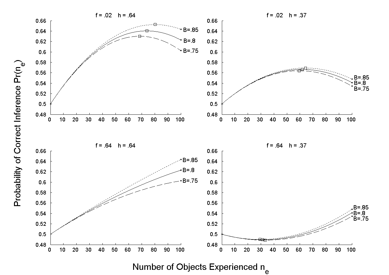
To allow comparison with the perfect-memory case where predictions were illustrated for α = 8, I set A = .8; B was set to .75, .8, and .85. Results were robust across z, so I set z = .5 . In Figure 2, there are illustrations of predicting and not predicting the less-is-more effect. In the two graphs of the upper panel, the full-experience effect is predicted: Accuracy is maximized at some amount of experience ne*, between 60 and 80, that is smaller than the full amount of experience N = 100. In the left graph of the lower panel, no less-is-more effect is predicted. In the right graph of the lower panel, the below-chance effect is predicted: Accuracy is higher at no experience ne,1 = 0 than at a larger ne,2 > 0, until ne,2 equals approximately 50.
Figure 2: Illustrations of conditions under which the less-is-more effect is and is not predicted. In all graphs, N = 100, z = .5 (results are robust across different values of z), A = .8, and B equals .75, .8, or .85. In the two graphs of the upper panel, a full-experience effect is predicted for f = .02 and h = .64 or .37 (the squares denote maximum accuracy). In the left graph of the lower panel, no less-is-more effect is predicted for f = h = .64. In the right graph of the lower panel, a below-chance effect is predicted for f = .64 and h = .37 (the squares denote minimum accuracy).
I now discuss other less-is-more effect predictions in the literature. Smithson (2010) analyzed a perfect- and an imperfect-memory model where knowledge consists of one cue. This implies that A and B are not necessarily constant across ne, contradicting Assumption 7; on the other hand, Smithson modeled h and f as probabilities constant across ne, agreeing with Assumption 6. He showed that the less-is-more effect can be predicted even if α ≤ β or A ≤ B. These results speak against the accurate-heuristics explanation. More specifically, Smithson also showed that the prediction of the less-is-more effect is largely influenced by aspects of memory such as the order in which objects are experienced and recognized and not so much on whether, or not, the experience and recognition heuristics are more accurate than recognition-based- or experience-based knowledge.
How can one reconcile Smithson’s and my results with Pleskac’s (2007) conclusion that A > B is necessary for the less-is-more effect when memory is imperfect? There are at least two ways. First, Pleskac studied a different model of imperfect memory from Smithson’s and the model presented here. In Pleskac’s model, recognition memory is assumed to be a Bayesian signal detection process. As a result of this assumption, the false alarm and hit rates are not constant across ne, thus contradicting Assumption 6 (which both models of Smithson and myself satisfy). On the other hand, in Pleskac’s model A and B are independent of ne, thus agreeing with Assumption 7 (which Smithson’s model does not satisfy). Second, Pleskac (2007) studied his model via simulations, and it could be that some predictions of the less-is-more effect, where it was the case that A ≤ B, were not identified.
This concludes the discussion of the theoretical predictions of the less-is-more effect. In the next section, I develop a method for testing them empirically.
In a task of forecasting which one of two national soccer teams in the 2004 European championship would win a match, Pachur and Biele (2007) did not observe the less-is-more effect even though “…the conditions for a less-is-more effect specified by Goldstein and Gigerenzer were fulfilled” (p. 99). Pohl (2006, Exp. 3) drew the same conclusion in a city-population-comparison task. The condition these authors mean is α > β (both values were averages across participants). Are these conclusions justified?
I do not think so, for at least two reasons. First, α > β is not the condition that should be tested. Second, even if it were, the estimates of and used are incorrect. Both complaints rely on the assumption that recognition memory is imperfect. If this assumption is granted, according to the analyses presented here one could test f < Kh/(1 − hz) or f > h/(1 − hz), but not α >β . Furthermore, the quantities used as estimates of α and β are estimates of complicated functions that involve A, B, h, f, n, and N. In the next paragraph I prove and illustrate this fact, and in the paragraph after that I use it to construct a new method for testing less-is-more-effect predictions.
Following Goldstein and Gigerenzer (2002), the αLit of a participant in an experiment has been estimated by the proportion of pairs where she recognized only one object, and in which the recognized object had a higher criterion value; and βLit has been estimated by the proportion of pairs where the participant recognized both objects, and in which she correctly inferred which object had a higher criterion value (the definitions are formalized in the result that follows). Result 3 shows what these estimates measure.
For the imperfect-memory model, (i) αLit = (p − q)A + pqB + (1 − p)(1 + q)(1/2); (ii) β Lit = p2 B + (1 − p)(1 + 3p)(1/2), where p = he/[he + f(1 − e)], q = (1 − h)e/[(1 − h)e + (1 − f )(1 − e)], e = (r − f )/(h − f ), and r = n/N.
Consider a participant. Let R be a recognized object and U an unrecognized object (both randomly sampled), with criterion values C(R) and C(U). Then, it holds that:
| αLit = Pr[C(R) > C(U)]. (4) |
Using the logic preceding the derivation of Equation (3), it also holds that:
Pr(C(R) > C(U) ∣ R is experienced, U is experienced) = B, Pr(C(R) > C(U) ∣R is experienced, U is not experienced) = A, Pr(C(R) > C(U) ∣R is not experienced, U is experienced) = 1 − A, Pr(C(R) > C(U) ∣R is not experienced, U is not experienced) = 1/2.(5) Let also:
|
Equations (4), (5), and (6)9 imply αLit = pqB + p(1 − q)A + (1 − p)q(1 − A) + (1 − p)(1 − q)(1/2), and this can be rewritten as in part (i) of the result.
Let R and R′ be recognized objects (both randomly sampled), with criterion values C(R) and C(R′). Also, assume that the participant infers that C(R) > C(R′). Then it holds that:
| βLit = Pr[C(R) > C(R′)]. (7) |
As in deriving (5), it holds that
Pr(C(R) > C(R′) ∣ R is experienced, R′ is experienced) = B and Pr(C(R) > C(R′) ∣ R is not experienced, R′ is not experienced) = 1/2. But we do not know Pr(C(R) > C(R′) ∣ R is experienced, , R′ is not experienced) and Pr(C(R) > C(R′) ∣ R is not experienced, R′ is experienced),because we do not know which of R and R′ has the higher criterion value. We can, however, reason that one of this probabilities equals A and the other one equals 1 − A.
From the above and Equation (7), it follows that βLit = p2B + (1 − p)2(1/2) + 2p(1 − p)(A + 1 − A), which can be rewritten as part (ii) of the result.
To complete the proof, I compute p and q. To do this, first let O be a randomly sampled object, and define e = Pr(O is experienced). Let also r = Pr(O is recognized), which, by definition, equals n/N. It holds that:
|
Solving the above equation for e, we get e = (r − f )/(h − f ).
Note that p = Pr(O is experienced ∣
O is recognized).
By Bayes’ rule, this probability equals
Pr(O is recognized ∣ O is experienced) ×
Pr(O is experienced)/Pr(O is recognized),
which turns out to be he/[he + f(1 − e)].
Similarly, q = Pr(U is experienced) =
Pr(O is experienced ∣ O is not recognized), and
this turns out to be (1 − h)e/[(1 − h)e + (1 − f )(1 − e)].
Because the estimates used can be determined from different experiments, it may be that some estimates are not well defined. For example, if h > r, then e > 1.
Result 3 says that the estimates of α and β used in the literature, αLit and βLit, are not straightforward to interpret. If memory is perfect, the estimates measure what they were intended to: f = 0 implies p = 1, and βLit = B = β = βe; if also h = 1, then q = 0, and αLit = A = α = αe. But if memory is imperfect, αLit may differ from αe, and βLit may differ from βe. Numerical illustrations of the difference between αLit and αe, and βLit and βe, are given in Table 2.
Table 2: Numerical illustration of the difference between αLit and αe, and βLit and βe, based on the average n, αLit, and βLit for each one of 14 groups in an experiment by Reimer and Katsikopoulos (2004), where participants had to compare the populations of N = 15 American cities. I also set h = .9, f =.1, and z = .5. For two groups, the estimates of αe were not between 0 and 1. On the average, αe was larger than αLit by .05, and βe smaller than βLit by .04.
n 9 12 10.3 12 11.3 13 11.3 12.3 9.3 12.3 10.7 12 8 9.7 αLit .79 .79 .78 .81 .88 .87 .72 .70 .68 .66 .79 .81 .77 .79 αe .81 .90 .80 .91 - - .75 .77 .68 .67 .83 .92 .79 .82 βLit .60 .58 .64 .62 .64 .66 .61 .60 .62 .64 .58 .60 .53 .54 βe .54 .55 .59 .59 .60 .63 .57 .57 .56 .61 .54 .57 .45 .49
In Table 2, I used the average n, αLit, and βLit for each one of 14 groups in an experiment by Reimer and Katsikopoulos (2004) where participants had to compare the populations of N = 15 American cities. I also set h = .9, f =.1, and z = .510. To compute αe and βe, I followed three steps: First, I computed p and q as in Result 3. Second, I solved for A and B from (i) and (ii) of Result 3, and B = [ βLit − (1 − p)(1 + 3p)(1/2)]/p2, A = [ αLit − pqB − (1 − p)(1 + q)(1/2)]/(p − q). Third, I used Equation (3) to compute αe and βe.
The difference between αLit and αe, or βLit and βe exceeded .01 in 24 out of 26 cases. The difference was as large as .11. On the average, αe was larger than αLit by .05, and βe was smaller than βLit by .0411. I also performed a sensitivity analysis, varying h from .9 to 1 in increments of .01 and f from .1 to 0 in decrements of .01. There were (14)112 = 1694 cases. On the average, αe was larger than αLit by .04, and βe was smaller than βLit by .02. One may expect these differences to increase if h and f are less indicative of a very good recognition memory than they were here.
Importantly, Result 3 implies that it is not straightforward to interpret the reported correlations between αLit and n, or βLit and n (Pachur & Biele, 2007; Pachur, in press). It is not clear that these correlations suggest substantial, or any, correlations between A and n, or B and n, because both αLit and βLit are complicated functions of n.
In fact, correlations between αLit and n, or βLit and n, are predicted even if A, B, h, and f are constant across n. For example, I computed the correlations between αLit and n, and βLit and n with the six parameter combinations used in the upper panel of Figure 2, where A = .8, B = .75, .8, or .85, h = .64 or .37, and f = .02 (N = 100). For each n from 0 to 100, I used the equations in the statement of Result 3 in order to compute αLit and βLit, and then computed their correlations with n.12
As can be seen in Table 3, correlations can be very substantial, varying from −.59 to .85. The average of the absolute value of the correlation between βLit and n is .65 (two correlations were negative and four were positive) and between αLit and n is .24 (all six correlations were negative).
Table 3: Numerical illustration of correlations between αLit and n, and LitβLit and n, even when A, B, h, and f are constant (N = 100). The average of the absolute value of the correlation between αLit and n is .65, and between LitβLit and n is .24.
Based on the points made in the previous paragraph, I claim that, unless it can be established that recognition memory was perfect in an experiment, a correct empirical test of the less-is-more effect in that experiment should not use the estimates of α and β in the literature (αLit and βLit).
There is one more problem with empirical tests of the less-is-more effect in the literature. The way some of these tests are carried out often provides no evidence for or against any theory of the conditions under which the less-is-more effect is predicted. To provide such evidence, it does not suffice to just check if an effect is found when the conditions in Results 1 or 2 are satisfied: Even if a condition for predicting the less-is-more effect holds, the prediction is not that all pairs of agents that have amounts of information n1 and n2 such that n1 < n2 would also have Pr(n1) < Pr(n2). For example, in the upper left panel of Figure 2, the less-is-more effect is predicted but it is also predicted that an agent who has experienced 40 objects would be less accurate than an agent who has experienced 100 objects. One cannot conclude that “no evidence for the less-is-more effect is found even if a condition that is sufficient for the effect holds”, in the case that a person who has experienced 40 objects is less accurate than another person who has experienced 100 objects.
For example, consider Pohl’s (2006) Experiment 3, which he interpreted as providing “no evidence for a less-is-more effect” (p. 262). For 11 German and 11 Italian cities, he measured the average, across participants, n, αLit, and βLit. Pohl observed that n was larger in German (11) than in Italian (9.5) cities, and αLit = .82, βLit = .74 for Italian cities; for German cities, αLit was not defined and βLit = .79. The less-is-more effect was not found: The accuracy for German cities (.78) was higher than the accuracy for Italian (.76) cities. But this is not evidence against the theory that, under the condition α > β, an effect is predicted: For the particular values of n, αLit, and βLit, applying Equation (2) does not predict a less-is-more effect, but rather that Pr(n) is higher for German (.79) than for Italian cities (.76), as it was indeed found.
In order to determine whether there is evidence for the less-is-more effect or not from an experiment, Snook and Cullen (2006), and Pachur and his colleagues (Pachur & Biele, 2007; Pachur, in press) searched for non-monotonic trends in the best-fitting polynomial to all data points {n, Pr(n)}. This partly addresses the issue I raised above because typically a large number of data points are considered, and it is likely that among them there are some pairs for which the effect is predicted. Remaining problems are that (i) the average prevalence and magnitude of the full-experience less-is-more effect are predicted to be small (see Table 1), and even the best-fitting polynomials of idealized curves are basically monotonic,13 and (ii) no out-of-sample-prediction criteria were used to identify these polynomials.
I now propose a method for testing the theoretical predictions of the less-is-more effect that avoids the issues discussed above and in the previous paragraph. The method consists of (i) computing the predicted accuracies of pairs of agents (individuals or groups), (ii) comparing the accuracies to determine whether a less-is-more effect is predicted or not, and (iii) checking the predictions against the observations. I first specify what data are assumed to be available.
A recognition experiment is one in which
αLit, βLit, n, and N are available.
All experiments in the literature run to test the less-is-more effect
are recognition experiments. The method uses the data of a recognition
experiment for each participant plus the values of three more
parameters, h, f, and z, which practically would often be
assumed equal for all participants. It may be fine to set z to a
fixed value, say .5 (because Pr(n) is robust across z). Currently,
estimates of h and f are not available from experiments run to
test the less-is-more effect. This is so because these experiments
used natural stimuli (e.g., cities) that participants had experienced
outside the laboratory. Estimates of h and f have to be taken from
the literature on tasks where experience is controlled, that are
similar to the task on which the test is based (e.g., recognition of
names, as in Jacoby et al., 1989).
The computation of the accuracy of an agent, Pr(ne), given αLit, βLit, n, N, h, f, and z, is a straightforward, albeit cumbersome, application of Result 3 and Equations (1) and (3):
αLit, βLit, n, N, h, f, and z.
r = n/N, e = (r − f )/(h − f ), p = he/[he + f(1 − e)], and q = (1 − h)e/[(1 − h)e + (1 − f )(1 − e)].
B = [ βLit − (1 − p)(1 + 3p)(1/2)]/p2, and A = [ αLit − pqB − (1 − p)(1 + q)(1/2)]/(p − q).
αe = (h − f + hfz)A +(1 − h + f − hfz)(1/2), and βe = h2B + (1 − h2)(1/2).
ne = (n − Nf )/(h − f ),
g(ne) = (N − ne)(N − ne − 1)/N(N − 1), r(ne) = 2 ne(N − ne)/N(N − 1), and k(ne) = ne(ne − 1)/N(N − 1).
Pr(ne) = g(ne)(1/2) + r(ne)αe + k(ne)βe.
Pr(ne).
I now illustrate the method. I use data from an experiment by Reimer
and Katsikopoulos (2004) where three-member groups had to perform a
population-comparison task with N = 15 American cities. In this
research, seven pairs of groups were identified so that (i) the
variability in n, αLit, and βLit across the three
group members was “small”, (ii) the difference in the average
αLit and βLit between the two groups in a pair was
“small”, and (iii) the difference in the average n between the two
groups in a pair was “large” (Reimer & Katsikopoulos, 2004,
pp. 1018-1019). I used the average n, αLit, and
βLit for each one of 14 groups (the values are provided in
Table 2). I also set h = .9, f =.1, and z = .5 (see comments in
Example 3).
Table 4: Numerical results of the method with data from Reimer and Katsikopoulos (2004; seven pairs of groups compared populations of N = 15 American cities). The method used the n, αLit, and βLit of this study (see Table 2), and h = .9, f = .1, z = .5 (see comments in Example 3), to predict Pr(ne). For one pair (3), the estimates of αe were not between 0 and 1, and the method was not applied. The less-is-more-effect predictions were correct for five pairs (1, 2, 4, 6, and 7) and incorrect for one pair (5).
Pair 1 Pair 2 Pair 3 Pair 4 Pair 5 Pair 6 Pair 7 n 9 12 10.3 12 11.3 13 11.3 12.3 9.3 12.3 10.7 12 8 9.7 Observed Pr(n) .83 .75 .73 .69 .78 .75 .67 .63 .66 .64 .67 .73 .56 .66 Predicted Pr(ne) .67 .64 .67 .66 - - .63 .60 .61 .61 .66 .66 .64 .65
In the Reimer-and-Katsikopoulos experiment, the less-is-more effect was observed in five out of the seven pairs (1-5) and not observed in two pairs (6, 7). As can be seen in Table 4, according to the method, the theory of the less-is-more effect, as summarized in Result 2, correctly predicts the effect in four pairs (1, 2, 4) and correctly predicts that there would be no effect in both pairs 6 and 714 (for one pair (3), the estimates of αe were not between 0 and 1, and the method was not applied). I also let h vary from .9 to 1 in increments of .01 and f vary from .1 to 0 in decrements of .01. The theory correctly predicted the effect in 402 out of 550 cases, correctly predicted no effect in 203 out of 242 cases, and was not applied in 55 cases. More generally, it should be studied further how robust the results of the method are when there is noise in the parameter estimates. This is a concern because of the nonlinear terms in various equations of the method.15
Strong predictions such as the less-is-more effect provide opportunities for theory development and deserve further study. This work made four contributions to the study of the less-is-more effect: Three refer to the theoretical predictions of the effect and one refers to how to empirically test these predictions.
First, I presented a characterization of the conditions under which the less-is-more effect is predicted (Result 2; this generalized the characterization of Goldstein & Gigerenzer, 2002). A main implication of the characterization is that it provides evidence against an implicit, but common explanation for the effect, the accurate-heuristics explanation (paragraph 3.3). The predictions were illustrated with parameter estimates from a recognition-memory experiment (Figure 2). Second, a new type of less-is-more effect, the below-chance effect, was predicted (paragraph 3.2). Third, I presented a simulation which showed that the less-is-more effect is predicted to be frequent, but its average magnitude is predicted to be small (Table 1), as it has been found empirically.
The fourth contribution was to point out some methodological issues in the empirical testing of less-is-more-effect predictions. In Result 3, it was shown that, granting that recognition memory is imperfect, the parameter estimates used in the tests are not measuring what they were intended to (Example 3). This result, however, allows constructing a new method for testing less-is-more-effect predictions (paragraph 4.2). Result 3 also has implications for the plausibility of the imperfect-memory model used here and of other models (Pleskac, 2007; Smithson, 2010). The main assumptions of my model (Assumptions 6 and 7) are independence assumptions: The parameters of the model (accuracies of the experience heuristic and knowledge, A and B, and probabilities of hits and false alarms, h and f ) are constant across information (the number of objects experienced, ne). These assumptions were made for mathematical convenience. Pleskac (2007) makes the independence assumption only for A and B and Smithson (in press) makes it only for h and f
Both authors have plausibility arguments against the independence assumptions they do not make: Pleskac appeals to a Bayesian signal detection model of recognition memory (for which he also cites studies that provide empirical support) that implies that h and f vary with ne, and Smithson constructs counterexamples where α and β vary with n, and A and B vary with ne.
These arguments have a lot to recommend them. But it is not clear how substantial the correlations have been found to be. Empirical evidence is provided by Pachur and colleagues (Pachur & Biele, 2007; Pachur, in press) who, across ten experiments, report average correlations between α and n, and between β and n, that range from .18 to .27. The problem is that the estimates of α and β used in these studies are not straightforward to interpret because they are estimates of complicated functions of A, B, h, f, N, and importantly, of n itself. In fact, I numerically showed (Table 3) that setting A, B, h, f, and N to be constant still led to correlations between the estimate of α used in the literature and n (.65, across six parameter combinations) and between the estimate of β used in the literature and n (.24). It seems that there is currently no definite evidence about which, if any, of the independence assumptions should be revised.
Unsatisfying at it is, my conclusion is that new and carefully controlled experiments are required in order to test the independence assumptions made here. Other empirical work I propose is to test the below-chance less-is-more effect. This effect requires below-chance recognition performance and it is not clear if it would be observed with natural and representative stimuli (Brunswik, 1954).
I end with a list of open questions for models of recognition memory that can be used in future theoretical work (Smithson, 2010, also has a list). A main question is which types of modeling assumptions are consistent with the enabling-of-accurate-heuristics explanation, and which are not. So far, we know that Pleskac’s assumptions seem to be consistent with this explanation, whereas the assumptions of Smithson and myself are not. Thus, the independence of the probabilities of hits and false alarms from experience could be key here. Other concepts that could be modeled are cognitive architecture (Schooler & Hertwig, 2005), familiarity (Dougherty et al., 2008), and learning and forgetting (Smithson, 2010).
Bishop, M. (2000). In praise of epistemic irresponsibility: How lazy and ignorant can you be? Synthese, 122, 179–208.
Broeder, A., & Schuetz, J. (2009). Recognition ROCs are curvilinear-or are they? On premature argument against the two-high-threshold model of recognition. Journal of Experimental Psychology: Learning, Memory, and Cognition, 35, 587–606.
Brunswik, E. (1955). Representative design and probabilistic theory in a functional psychology. Psychological Review, 62, 193–217.
Busemeyer, J. R. (1993). Violations of the speed-accuracy tradeoff relation: Decreases in decision accuracy with increases in decision time. In O. Svenson and A. J. Maule (Eds.), Time Pressure and Stress in Human Judgement and Decision Making (pp. 181–193). New York: Plenum Press.
Davis-Stober, C. P., Dana, J., & Budescu, D. V. (2010). Why recognition is rational: Optimality results on single-variable decision rules. Judgment and Decision-Making, 5, 216–229.
Dawes, R. M., & Corrigan, B. (1974). Linear models in decision making. Psychological Bulletin, 81, 95–106.
Dougherty, M. R., Franco-Watkins, A. M., & Thomas, R. (2008). Psychological plausibility of the theory of probabilistic mental models and the fast and frugal heuristics. Psychological Review, 115, 119–213.
Garrett, H. E. (1922). A study of the relation of accuracy to speed. Archives of Psychology, 56, 1–104.
Gigerenzer, G., Todd, P. M., and the ABC Research Group (1999). Simple Heuristics that Make us Smart. New York: Oxford University Press.
Goldstein, D. G., & Gigerenzer, G. (2002). Models of ecological rationality: The recognition heuristic. Psychological Review, 109, 75–90.
Hertwig, R., Herzog, S. M., Schooler, L. J., & Reimer, T. (2008). Fluency heuristic: A model of how the mind exploits a by-product of information retrieval. Journal of Experimental Psychology: Learning, Memory, & Cognition, 34, 1191–1206.
Hertwig, R., & Todd, P. M. (2003). More is not always better: The benefits of cognitive limits. In D. Hardman and L. Macchi (Eds.), Thinking: Psychological Perspectives on Reasoning, Judgment, and Decision Making, Chichester, UK: John Wiley and Sons.
Hick, W. E. (1952). On the rate of gain of information. Quarterly Journal of Experimental Psychology, 4, 11–26.
Hogarth, R. M., & Karelaia, N. (2005). Ignoring information in binary choice with continuous variables: When is less "more"? Journal of Mathematical Psychology, 49, 115–124.
Jacoby, L. L., Woloshyn, V., & Kelley, C. (1989). Becoming famous without being recognized: Unconscious influences of memory produced by dividing attention. Journal of Experimental Psychology, 118, 115–125.
Katsikopoulos, K. V., & Martignon, L. (2006). Naïve heuristics for paired comparisons: Some results on their relative accuracy. Journal of Mathematical Psychology, 50, 488–494.
Koutstaal, W., & Schacter, L. D. (1997). Gist-based false recognition of pictures in younger and older adults. Journal of Memory and Language, 37, 555–583.
Pachur, T. (in press). Inferences based on the recognition heuristic: Is less more in the real world? Psychonomic Bulletin and Review.
Pachur, T., & Biele, G. (2007). Forecasting from ignorance: The use and usefulness of recognition in lay predictions of sports events. Acta Psychologica, 125, 99–116.
Pachur, T., Mata, R., & Schooler, L. J. (2009). Cognitive aging and the adaptive use of recognition in decision-making. Psychology and Aging, 24, 901–915.
Pleskac, T. J. (2007). A signal detection analysis of the recognition heuristic.Psychonomic Bulletin and Review, 14, 379–391.
Pohl, R. F. (2006). Empirical tests of the recognition heuristic. Journal of Behavioral Decision Making, 19, 251–271.
Reimer, T., & Katsikopoulos, K. V. (2004). The use of recognition in group decision-making. Cognitive Science, 28, 1009–1029.
Roediger, H. L. (1996). Memory illusions. Journal of Memory and Language, 35, 76–100.
Roediger, H. L., & McDermott, K. B. (1995). Creating false memories: Remembering words not presented in lists. Journal of Experimental Psychology: Learning, Memory, and Cognition, 21, 803–814.
Schooler, L. J., & Hertwig, R. (2005). How forgetting aids heuristic inference. Psychological Review, 112, 610–628.
Shepard, R. N. (1967). Recognition memory for words, sentences, and pictures. Journal of Verbal Learning and Verbal Behavior, 6, 156–163.
Smithson, M. (2010). When less is more in the recognition heuristic. Judgment and Decision-Making, 5, 230–243.
Snook, B., & Cullen, R. M. (2006). Recognizing national hockey league greatness with an ignorance-based heuristic. Canadian Journal of Experimental Psychology, 60, 33–43.
Trafimow, D. (2003). Hypothesis testing and theory evaluation at the boundaries: Surprising insights from Bayes’s theorem. Psychological Review, 110, 526–535.
This document was translated from LATEX by HEVEA.