Judgment and Decision Making, vol. 5, no. 4, July 2010, pp. 216-229
Why recognition is rational: Optimality results on single-variable decision rulesClintin P. Davis-Stober* |
The Recognition Heuristic (Gigerenzer & Goldstein, 1996; Goldstein & Gigerenzer, 2002) makes the counter-intuitive prediction that a decision maker utilizing less information may do as well as, or outperform, an idealized decision maker utilizing more information. We lay a theoretical foundation for the use of single-variable heuristics such as the Recognition Heuristic as an optimal decision strategy within a linear modeling framework. We identify conditions under which over-weighting a single predictor is a mini-max strategy among a class of a priori chosen weights based on decision heuristics with respect to a measure of statistical lack of fit we call “risk”. These strategies, in turn, outperform standard multiple regression as long as the amount of data available is limited. We also show that, under related conditions, weighting only one variable and ignoring all others produces the same risk as ignoring the single variable and weighting all others. This approach has the advantage of generalizing beyond the original environment of the Recognition Heuristic to situations with more than two choice options, binary or continuous representations of recognition, and to other single variable heuristics. We analyze the structure of data used in some prior recognition tasks and find that it matches the sufficient conditions for optimality in our results. Rather than being a poor or adequate substitute for a compensatory model, the Recognition Heuristic closely approximates an optimal strategy when a decision maker has finite data about the world.
Keywords: improper linear models, recognition heuristic, single-variable decision rules.
Common sense would suggest that it is always better to have more, rather than less, relevant information when making a decision. Most normative and prescriptive theories of multi-attribute decision making are compensatory models that incorporate all relevant variables. This perspective was challenged by Gigerenzer and Goldstein (1996) and Gigerenzer, Todd, and the ABC Group (1999), who proposed a theoretical framework of simple decision rules, often referred to as “fast and frugal” heuristics, suggesting that in some cases a decision maker (DM) utilizing less relevant information may actually outperform an idealized DM utilizing all relevant information. In fact, many of these heuristics use a single cue selected among the many available for the prediction task. Key among these single-variable decision rules is the Recognition Heuristic (RH) (Gigerenzer & Goldstein, 1996; Gigerenzer et al., 1999; Goldstein & Gigerenzer, 2002).
A rapidly growing empirical literature suggests that single-variable decision rules are descriptive for at least a subset of DMs with regard to both Take The Best (Bröder, 2000; Bröder & Schiffer, 2003; Newell & Shanks, 2003) and the RH (Goldstein & Gigerenzer, 2002; Hertwig & Todd, 2003; Pachur & Biele, 2007; Scheibehenne & Bröder, 2007; Serwe & Frings, 2006; Snook & Cullen, 2006). Questions remain, however, as to exactly when and why a single-variable rule will perform well.
Hogarth and Karelaia (2005) examined the relative performance of single-variable rules within a binary choice framework where both predictor (independent) and criterion (dependent) variable were assumed to be continuous. Using a combination of analytic tools and simulations, they found that single-variable rules have strong predictive accuracy when: 1) all predictors are highly and positively inter-correlated, 2) the single predictor used is highly (and, typically, positively) correlated with the criterion.1 Hogarth and Karelaia (2006) conducted a related analysis using binary rather than continuous cues (predictors). Fasolo, McClelland, and Todd (2007) identified similar favorable conditions for single-variable rules using a series of simulations. Shanteau and Thomas (2000) labeled environments with highly positively correlated predictors, “friendly” environments, and demonstrated in a simulation that single-variable rules tended to underperform when the predictors in the model were negatively correlated, a finding that was later replicated by Fasolo et al. (2007) (see also Martignon & Hoffrage, 1999; and Payne, Bettman, & Johnson, 1993). In a similar vein, Baucells, Carrasco, and Hogarth (2008) presented a framework to analyze simple decision rules within the context of cumulative dominance (see also Katsikopoulos & Martignon, 2006).
In this paper, we present results regarding the effectiveness of single variable rules that diverge from previous studies in two major ways. First, we show that when a single predictor, denoted without any loss of generality, x1, is positively correlated with an array of p-many other predictors, where each of these p-many predictors are either uncorrelated or weakly positively correlated, the optimal weighting scheme places greater weight on x1 than any of the remaining cues. This result is a major departure from previous studies (Fasolo et al., 2007; Hogarth & Karelaia, 2005; Shanteau & Thomas, 2000) that identify favorable conditions for single-variable rules as “single-factor” models where all variables are highly positively correlated. Second, our results do not rely on any specific assumptions about the cue validities, defined as the correlations between the predictors (cues) and the criterion. The only thing that matters is the sign on the correlation of the single cue. Some lexicographic single-variable rules depend upon either the knowledge or estimation of all cue validities. For example, the Take The Best rule (Gigerenzer & Goldstein, 1996; Gigerenzer et al., 1999) depends on the identification of the single best cue. In our results, the validity of the single variable need not be the highest among the available predictors. We apply the new results to the RH, for which Goldstein and Gigerenzer (2002) argue that the recognition validity, i.e., the correlation between the criterion and recognition, is inaccessible to the DM with the criterion variable influencing recognition through mediator variables in the environment.
The divergence in our results stems from our somewhat different approach to answering the question “when does less information lead to better performance?” First, we characterize the RH within the framework of the linear model — i.e., within the standard regression framework — as an “estimator” that relies on a single predictor. As in the regression framework, we conceptualize the best set of weights to assign to the cues, such that if one had unlimited data and knowledge, they would maximize predictive accuracy and call this vector of weights β. We then consider the weights that would be placed on the cues by various decision heuristics (such as equal weighting) as if they were estimates of β. Within this framework, we can prove results with respect to a measure of statistical inaccuracy called “risk” (defined formally in section 2), which measures how close these heuristic weights are expected to be to the best weights, β. This measure of inaccuracy is particularly useful because it goes beyond optimizing within a single sample; the closer a set of weights is to the best weights, the more robustly it cross-validate in new samples. An advantage to casting the problem within the framework of the linear model is that the results can be generalized to accommodate a broad range of situations, including choosing between more than two options, binary or continuous representations of recognition, and to evaluate the success of any single variable rule, not just RH.
We show that under certain conditions, placing greater weight on a single variable relative to all others represents a form of optimization: It minimizes the maximum value of risk over all choices of decision rules. As the number of cues becomes large, this mini-max strategy converges to a rule that puts a large weight on a single cue and minimally weights all others. We use the term “over-weighting” to describe this effect of a single predictor cue receiving disproportionally more weight than any other predictor cue according to an optimal weighting strategy. Further, we show that weighting the single cue and ignoring all others produces the same risk as ignoring the single cue and weighting all others, regardless of the number of cues. Previous research has shown that decision heuristics applied in this manner outperform standard regression models until samples become very large (Davis-Stober, Dana, & Budescu, 2010). Thus we expect that, under the right conditions, a single variable to be just as accurate a predictor as the full set of predictors.
While this framework could be used to justify any single variable heuristic, we argue that the sufficient conditions plausibly resemble environments in which one would use the RH, and where recognition is the single cue. Indeed, we examine data used in prior recognition tasks (Goldstein, 1997) and show that it fits well our sufficient conditions. Our derivation does not assume a “cue selection” process. In other words, we presuppose the DM always utilizes the single cue of interest. The RH theory is a natural application of these results as this theory also does not presuppose a cue selection process, i.e., if one alternative is recognized and the other is not then recognition is automatically the predictor cue of interest.
Why is recognition rational? Our results demonstrate that when a single cue (recognition) is positively correlated with all other cues (knowledge), then it is a mini-max strategy to over-weight the recognition cue. Interestingly, these results do not depend upon the validities of either the recognition or the knowledge cues.
This paper represents a convergence of two perspectives. On the one hand, we validate the ecological rationality of single variable rules by recasting them as robust statistical estimators that minimize maximal risk within a linear model. From another perspective, our results suggest that the heuristics could work for no other reason than that they approximate an optimal statistical model, albeit with an objective function that has heretofore been unarticulated in this literature. Thus, while Goldstein and Gigerenzer (2002) see the RH approach as a contrast to heuristics being used as “imperfect versions of optimal statistical procedures,” it appears that the “Laplacean demon” (Gigerenzer & Goldstein, 1996; Todd, 1999) — with unlimited computational power — would use a rule much like the RH!
The remainder of the paper is organized as follows. First, we summarize recent advances on the evaluation of decision heuristics within the linear model and make some simplifying assumptions. We then describe the sufficient conditions for the single-variable “over-weighting” phenomenon, first considering the case of a single variable correlated with an array of weakly positively inter-correlated predictors followed by the more extreme case of a set of mutually uncorrelated predictors within this array. We then present an application of this theory to the RH and prove that under these conditions a DM utilizing only recognition will perform at least as well as a DM utilizing only knowledge. We then examine the inter-correlation matrix of an empirical study, finding preliminary support for the descriptive accuracy of these sufficient conditions. We conclude with a summary and discussion of these results and potential applications and implications.
We consider decision heuristics as a set of weighting schemes embedded within the linear model, a standard formulation when evaluating performance, e.g., when one compares performance to that of regression (e.g., Martignon & Hoffrage, 2002; Hogarth & Karelaia, 2005). Specifically, we re-cast decision heuristics as “improper” linear models (Dawes, 1979) within a linear estimation framework, treating each weighting scheme as an estimator of the true relationship between the criterion and the predictors. This formulation allows us to evaluate different weighting schemes by a standard statistical measure of performance, risk, utilizing recent advances in the evaluation of “improper” models (Davis-Stober et al., 2010).
The standard linear model is defined as:
| Yi = |
| βjxij + єi, (1) |
where єi ∼ (0,σ2). We include p+1 predictors to distinguish between the single predictor and the other p. In this paper, we use the linear model interchangeably as either a representation of a criterion (target) variable with environmental predictors or as a representation of a DM’s utility for choice alternative Ci (Keeney & Raiffa, 1993), which can be expressed as:
| U(Ci) = |
| βjxij + єi. (2) |
In this case, the weights, βj, reflect a DM’s true underlying utility. The results in this paper are general and can be applied to model either the environment (1) or the individual (2). The environmental case (1) is particularly applicable to recognition. In this case, the performance of an individual DM is a function of the true underlying relationship between recognition, environmental cues, and the criterion of interest.
For either case, we are interested in examining different estimators of β, denoted by the vector β. We apply the standard statistical benchmark, risk, to assess the performance of an estimator of the “true” relationship between a criterion and predictors. Risk for an estimator β is defined as
| Risk(β) = E||β − β||2, (3) |
where E is the expectation of a random variable and ||β − β||2 is the sum of squared differences between the coefficients of β and β. Informally, (3) is a measure of how “far” an estimator is expected to be to the “true” value of β. Risk (also known in the literature as the Mean Squared Error or MSE) can be decomposed into the squared bias of the estimates and their variance. Unlike other criteria that focus on unbiasedness, risk minimization provides a more flexible framework where bias and variability are traded off. In many cases estimates with relatively low bias can reduce considerably the variance and would be considered superior with respect to their overall risk. This definition of risk allows us to directly compare fixed weighting schemes to other statistical estimators, and to each other. Our definition of risk bears some qualitative similarity to the “matching” index (Hammond, Hursch, & Todd, 1964) applied to the well-known lens model (Brunswik, 1952). It is a measure of fit between a person’s judgment, or choice of weights, and an optimal weighting scheme within the environment.
To compare various weighting schemes within the context of the linear model, we use what are commonly referred to as “improper” linear models (Dawes, 1979; Dawes & Corrigan, 1974). These are fixed and pre-determined weighting schemes which are chosen independently of the data collected. Let a denote an improper weighting vector. An example would be “Dawes Rule,” where a is a vector of all ones (Dawes, 1979). In this example, the weights βj in (1) and (2) are replaced with ones, resulting in an equal weighting of all the predictors (these predictors are typically assumed to be standardized and/or properly calibrated). When considered as estimators, improper models are clearly both biased and inconsistent, yet many of these a priori weighting schemes have been shown to be surprisingly accurate. For example, Wainer (1976) and Dawes (1979) have demonstrated the excellent predictive accuracy of equally weighting all predictors in a linear regression model.
We are interested in examining various choices of weights, a, using the criterion of risk (see (3)). To proceed, we re-cast the weighting vector a as a statistical estimator of β. Davis-Stober et al. (2010) define a constrained linear estimator, βa, as
| βa = a(a′X′Xa)−1a′X′y, (4) |
where X is the matrix that consists of the values of all p+1 predictors for all n cases, and y is a series of n observations of the criterion (target) variable Y in (1) and (2).
The constrained estimator (4) is a representation of the “improper” weighting scheme, a, in the sense that it is the least-squares solution to the estimation of β subject to the constraints in a. In other words, if the weighting scheme a is a vector of ones (i.e., equal weights) then βa1 = βa2 = βa3 = … = βa(p + 1). The reader should note that while data are being used to scale the weighting vector a in (4), the resulting coefficient of determination, R2, is the same as if only a had been used (because R2 is invariant under linear transformation). Thus, this formulation will not affect the outcomes in the binary choice task considered, nor would it ever change a DM’s ranking of several objects on the criterion. The formulation in (4), however, allows us to define and compute an upper bound on the maximal risk for arbitrary choices of the weighting vector a.
Given a choice of weighting vector a and design matrix X, Davis-Stober et al. (2010) proved that the maximal risk of (4) is as follows,
| maxRisk(βa) = ||β||2 | ⎛ ⎜ ⎜ ⎝ |
| ⎞ ⎟ ⎟ ⎠ | + |
| , (5) |
where ||β||2 denotes the sum of squared coefficients of β. Equation (5) allows us to measure the performance of a particular choice of a. Davis-Stober et al. (2010) provide an analysis of (5) for several well-known choices of a, including: equal weights (Dawes, 1979), weighting a subset of cues while ignoring others, and unit weighting (Einhorn & Hogarth, 1975).
It is often useful, given a choice of X, to know the
optimal choice of weighting vector a.
Davis-Stober et al. (2010) prove that the value of weighting vector
a that minimizes maximal risk is the
eigenvector corresponding to the largest eigenvalue in the matrix
X′X.
Theorem (Davis-Stober et al., 2010).
Define λmax as the largest eigenvalue of the matrix
X′X. Assume ||β||2 <
∞. The weighting vector a that is mini-max with
respect to all a ∈ ℝp+1, is the eigenvector
corresponding to the largest eigenvalue of X′X.
In other words, given a model of the matrix X′X, it is
possible to identify the fixed weighting scheme that minimizes maximal
risk. Remarkably, this optimal weighting scheme does not depend on the
individual predictor cue validities.
To summarize, each choice of weighting scheme, a, can be considered as an estimator of β in the linear model using (4). We can compute an upper bound on the maximal risk that each choice of a will incur using (5). Finally, given a model of X′X, we can calculate the optimal choice of weighting vector a using the above theorem. In the next section, we apply these results to the case of a single predictor cue positively inter-correlated with an array of p-many other predictor cues, all of which are weakly positively inter-correlated and, in the limit, mutually uncorrelated.
Henceforth, assume that all the variables are
standardized such that Xi = 0 and sXi2 =
1 for all i. This implies that X′X =
(n−1)RXX, where n is the sample size and
RXX is the correlation matrix of the predictor
variables. Let rij denote the the (i,j)th entry of
RXX. For our analysis of single variable rules, we
are interested in the case when there are a total of (p+1)-many
predictors, where p-many predictors follow a “single-factor”
design, i.e., all p-many predictors in this array are assumed to be
inter-correlated at r′ with the remaining predictor equally
inter-correlated with all other predictors at r.
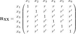
Condition 1. Assume that RXX is
comprised of p+1 predictor cues, p-many of which are
inter-correlated at r′ with the remaining predictor cue correlated
with all others at r. Assume r > 0 and r′ ≥ 0.
For the case of p=5, Condition 1 specifies the following correlation matrix.
This structure is a special case of the two-factor oblique correlation matrix presented in Davis-Stober et al. (2010). Davis-Stober et al. (2010) provided a closed-form solution for all eigenvalues and corresponding eigenvectors of this matrix. Applying those results we obtain the maximum eigenvalue for matrices satisfying Condition 1 as
| λmax = |
| ⎛ ⎜ ⎝ | 2 + (p − 1)r′ + | √ |
| ⎞ ⎟ ⎠ | , |
with a corresponding (un)-normed eigenvector with the first entry valued at
| , |
with the remaining p-many entries valued at 1. Applying the
previous theorem, we can now state precisely the mini-max choice of
weighting scheme for matrices satisfying Condition 1.
Result 1. Assume the matrix structure described in
Condition 1.
Let c = p + (√((p−1)r′)2 + 4pr2 −(p − 1)r′)2/4r2 . The normed choice of weighting vector that is mini-max with respect to risk, denoted a*, is:
| a* = [ |
| , |
| , |
| , |
| , |
| , … |
| ]. (6) |
Note that the relative weights of the predictors are unchanged by scalar multiplication.
Figure 1: This figure displays the ratio a1*/ai* as a function of r and p under Condition 1 with r′ = .3. 
Result 1 presents the mini-max choice of a fixed weighting vector for the inter-correlation matrix specified in Condition 1. In other words, given a linear model structure as in (1)–(2) and assuming the inter-correlation matrix of the predictor cues follow the structure in Condition 1, then (6) is the best choice of fixed weighting scheme with respect to minimizing maximal risk. This leads to an important question. Assuming Condition 1 holds, when will it be a mini-max strategy to place more weight on a single predictor cue (in our case x1) than any other cue? The next result answers this question.
Result 2. Assume RXX is defined
as in Condition 1. Let a* be the mini-max choice of
weighting scheme (Equation 6). Let ai* denote the ith
element of the vector a*. Then a1*>
ai*, ∀ i ∈ {2, 3, …, p+1}, if, and only if,
r>r′.
Proof. Applying Result 1, a1*> ai*,
∀ i ∈ {2, 3, …, p+1}, if, and only if, p −
r′/r(p−1) > 1, which implies that r>r′. □.
Result 2 states that it is an optimal mini-max strategy, with respect
to risk, to overweight a single predictor when that single predictor
positively correlates with the other predictors, which are weakly
positively2 inter-correlated or
mutually uncorrelated. Result 2 suggests that the overweighting
effect of the first predictor becomes more pronounced as the ratio
r′/r becomes small and/or as the number of
predictors increase. Figure 1 plots the ratio
a1*/ai* as a function of p and r for a fixed
value of r′ = .30. As expected, the relative weight placed
on the first predictor increases smoothly as a function of both
p and r.
As an example, let p = 5, r=.6, r′ = .25. This gives the following
matrix for six predictors.
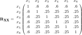
RXX has the following mini-max choice of a,
| a* = [ .57 .37 .37 .37 .37 .37 ]. |
In this example, the first element in the mini-max choice of weighting scheme, a1*, is over one and half times as large as the remaining weights. This overweighting effect becomes even more pronounced when the predictors in this p-element array are mutually uncorrelated.
In contrast to the conditions identified in Hogarth and Karelaia
(2005) and Fasolo et al. (2007), this over-weighting effect becomes
more pronounced as both the number of predictors increase and the
inter-correlations of the p-many predictor array approach 0. In
this section, we analyze the extreme case of a single cue positively
correlated with p-many predictors which are mutually
uncorrelated. This is a special case of Result 2 when r′ = 0. In
the asymptotic case, where the number of predictors is unbounded, the
weights on the p-many predictors become arbitrarily small.
Condition 2. Let RXX be defined
as in Condition 1 and assume r′=0.
Condition 2 is a special case of Condition 1 so, applying Result 1,
the maximal eigenvalue of RXX under Condition 2 is
equal to
| λmax = 1 + r | √ |
| , |
and the corresponding normed eigenvector (and the mini-max choice of a) equals
| a* = [ |
|
|
|
|
| … |
| ]. (7) |
It is easy to see that as the number of predictors increases, i.e., as p becomes large, the weights on the p-many predictor cue entries come arbitrarily close to 0 while a1* remains constant.
Put another way, when r′=0, it is mini-max with respect to risk for
a decision maker to heavily weight the single predictor. The
effectiveness of this strategy becomes more pronounced as the number
of mutually uncorrelated predictors increases.
As a numerical example, let p = 5, r′ = 0. This gives the following
matrix for six predictors.
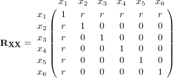
RXX has the following mini-max choice of a,
| a* = [ .71 .32 .32 .32 .32 .32 ]. |
For this example, the weight on x1 is more than double the weight of each of the other predictors. In general, the ratio, a1*/ai* = √p. Thus, if for example, p = 100, the weight on x1 would be 10 times as large as the weight on any other predictor. We emphasize that the mini-max choice of weighting under Condition 2 does not depend upon the value r.
The preceding results are a mathematical abstraction, in the sense that typically all predictors are neither equally correlated, nor mutually uncorrelated. However, it is clear from these derivations that this over-weighting effect of a single variable, with respect to risk, will occur whenever the single variable of interest is positively correlated with the other predictors and this correlation dominates the inter-correlations of the remaining predictors. In the next section we demonstrate how this over-weighting effect applies to the performance of the Recognition Heuristic, showing that under Condition 2 a DM using only recognition will perform as well as a DM using only knowledge.
The RH is arguably the simplest of the “fast and frugal” heuristics that make up the “adaptive cognitive toolbox” (e.g., Gigerenzer et al., 1999). Quite simply, if a DM is choosing between two alternatives based on a target criterion, the recognized alternative is selected over the one that is not. Goldstein and Gigerenzer (2002) state that a “less-is-more effect” will be encountered whenever the probability of a correct response using only recognition is greater than the probability of a correct response using knowledge (equations (1) and (2) in Goldstein & Gigerenzer, 2002), in their words: “whenever the accuracy of mere recognition is greater than the accuracy achievable when both objects are recognized.” Goldstein and Gigerenzer’s conditions for the success of the recognition heuristic depend upon the recognition validity, i.e., the correlation between the target criterion and recognition, which is assumed not to be directly accessible to the DM. Other environmental variables, called mediator variables, which are positively correlated with both the target criterion (the ecological correlation) and the probability of recognition (the surrogate correlation), influence the DM as proxies for the target criterion. We build upon the recognition heuristic theory by defining a condition on the predictor cues that leads to a mini-max strategy closely mirroring the recognition heuristic. Conditions 1 and 2 depend only upon observable predictor cue inter-correlations and do not require the estimation or assumption of either a recognition validity or corresponding surrogate and ecological correlations.
In this section we present a linear interpretation of the recognition heuristic by defining weighting schemes representing a DM using only recognition or only knowledge. We present a proof (Result 3) that a DM using only recognition will incur precisely the same amount of maximal risk as a DM using only knowledge under Condition 2. This result states that a DM using only recognition will do at least as well as using only knowledge with respect to maximal risk. We compare these weighting schemes to each other, the optimal mini-max weighting, and Ordinary Least Squares (OLS).
To apply the optimality results presented above, we must first re-cast the RH within the linear model. Let xi1 be the recognition response variable with respect to the RH theory. Let the remaining p-many predictors correspond to an array of predictors relevant to the criterion under consideration. Within the RH framework, we shall refer to these p-many variables as knowledge variables. This gives the following model,
| Yi = |
| + |
| + |
| . (8) | |||||||||||||||||||||||||||||||||||||||||||||||||||||||||||
The recognition variable, xi1, is typically conceptualized as a binary variable (e.g., Goldstein & Gigerenzer, 2002). Pleskac (2007) presents an analysis of the recognition heuristic in which recognition is modeled as a continuous variable integrated into a signal detection framework (see also Schooler and Hertwig, 2005). Note that our general result on maximal risk (5) holds for an arbitrary matrix, X, in which predictor cues can be binary, continuous or any combination of the two types.
We use maximal risk as the principal measure of performance within the linear model, in contrast to previous studies that used percentage correct within a two-alternative forced choice framework as a measure of model performance (e.g., Goldstein & Gigerenzer, 2002; Hogarth & Karelaia, 2005). As such, we do not compare individual values of Y for different choice alternatives. We instead make the assumption that a DM using “true” β as a weighting scheme will outperform a DM using any other choice of weighting scheme. In our framework, minimizing maximal risk corresponds to a DM using a fixed weighting scheme that is “closer” to the “true” β compared to any other fixed weighting scheme.
The Recognition Heuristic assumes that the DM can find him/herself in one of three mutually exclusive cases, that induce different response strategies: 1) neither alternative is recognized and one must be selected at random, 2) both alternatives are recognized and only knowledge can be applied to choose one of them, and 3) only one alternative is recognized (the other is not), so the DM selects the alternative that is recognized. To model this process, we consider the following two choices of the weighting vector a:
In the context of the linear model (8), the act of recognizing an item but having no knowledge of that item is modeled by aR, i.e., recognizing one choice alternative without applying knowledge to the decision. The act of only using knowledge to select between items is modeled by aK, corresponding to a DM recognizing both choice alternatives and relying exclusively on knowledge to make the decision. We do not analyze the trivial case of neither alternative being recognized. To facilitate comparison of these weights, let aM be the mini-max weighting scheme from Result 1 and let OLS be the ordinary least squares estimate.
Figure 2: This figure displays the maximal risk as a function of sample size for four choices of weighting schemes: aR (solely recognition), aK (solely knowledge), aM (mini-max weighting), and OLS (ordinary least squares). These values are displayed under Condition 1, where r′= .25, r = .6, p = 6, and σ2 = 2. The left-hand graph displays these values assuming R2 = .3. The center and right-hand graphs display these values for R2 =.4 and R2 = .5 respectively.
We can now describe and analyze when “less” information will lead to
better performance in the language of the linear model. When will
aR perform as well as, or better, than
aK? Consider Condition 2, i.e., the case when the
p-many predictor cues are mutually independent, r′=0. Under these
circumstances the over-weighting effect of the mini-max vector is most
pronounced and, surprisingly, the weighting schemes
aR and aK incur exactly the
same amount of maximal risk.
Result 3. Let RXX be defined as
in Condition 2, i.e., r′ = 0. Let aR and
aK be defined as above. Then max
Risk(aR) = maxRisk(aK).
Proof. The proof follows by direct calculation using (5),
| maxRisk(βaR) = ||β||2 | ⎛ ⎜ ⎜ ⎝ |
| ⎞ ⎟ ⎟ ⎠ |
| + |
|
| = ||β||2(pr2 + 1) + σ2 |
| = ||β||2 | ⎛ ⎜ ⎜ ⎝ |
| ⎞ ⎟ ⎟ ⎠ | + |
|
| = maxRisk(βaK). □ |
Result 3 provides a new perspective on the phenomenon of “less”
information leading to better performance: A simple single-variable
decision heuristic (e.g., the recognition heuristic) is at least as
good in terms of risk as equally weighting the remaining cues, e.g.,
knowledge.
Figure 3: This figure displays the maximal risk as a function of sample size for four choices of weighting schemes: aR (solely recognition), aK (solely knowledge), aM (mini-max weighting), and OLS (ordinary least squares). These values are displayed under Condition 2, where r′= 0, r = .3, p = 3, and σ2 = 2. The left-hand graph displays these values assuming R2 = .3. The center and right-hand graphs display these values for R2 = .4 and R2 = .5 respectively.
We can directly compare the performance of aK, aR, aM, and OLS by placing some weak assumptions on the intercorrelation matrix of the predictors and the values of σ2 and ||β||. First, we can bound ||β||2 by applying the inequality ||β||2 ≤ R2/λmin, where R2 is the coefficient of multiple determination of the linear model and λmin is the smallest eigenvalue of the matrix RXX. Now, assuming values of σ2, R2, and a structure of RXX we can compare the maximal risk for different weighting vectors as a function of sample size. Under our framework, sample size does not play a role in determining the mini-max choice of fixed weighting scheme, however we must consider sample size when comparing values of risk to other estimators, in this case OLS.
How do recognition and knowledge compare with the mini-max choice of weighting scheme? Figure 2 displays the maximal risk for aK, aR, aM, and OLS, under Condition 1 for p=6, r=.6, r′ = .25, and σ2 = 2. The three panels of Figure 2 corresponds to R2 = .3, .4, and .5.
The performance of the knowledge, recognition, and mini-max weighting are comparable in all three conditions with the knowledge weighting, aK, coming closest to the optimal weighting scheme. In the case of Condition 1, recognition does not win out over knowledge, however recognition wins out over OLS for sample sizes as large as n = 30 in the case of R2 = .3 and n = 20 for the case of R2 = .5.
Figure 3 displays a corresponding set of graphs under Condition 2 for p=3, r=.3, r′ = 0, and σ2 = 2. As predicted by Result 3, recognition and knowledge have precisely the same maximal risk. The mini-max weighting scheme is quite comparable to knowledge/recognition performance. The performance of OLS improves in Condition 2; this follows from the matrix X′X having fewer inter-correlated predictors.
To summarize, under Condition 1, both recognition and knowledge compare favorably to OLS and to the mini-max choice of weighting. Here recognition does not perform as well as knowledge but is comparable. Under Condition 2, the maximal risk of recognition and knowledge are identical, as shown in Result 3, and closely resemble the performance of the mini-max choice of weighting vector. In all cases, the performance of the different weighting schemes are affected by the amount of variance in the error term єi, in agreement with Hogarth and Karelaia (2005).
Table 1: Predictor Cues for the “German Cities” Study (Gigerenzer et al., 1999; Goldstein, 1997).
Cue description Predictor Cue Recognition x1 National capital (Is the city the national capital?) x2 Exposition Site (Was the city once an exposition site?) x3 Soccer team (Does the city have a team in the major leagues?) x4 Intercity train (Is the city on the Intercity line?) x5 State capital (Is the city a state capital?) x6 License plate (Is the abbreviation only one letter long?) x7 University (Is the city home to a university?) x8 Industrial belt (Is the city in the industrial belt?) x9 East Germany (Was the city formerly in East Germany?) x10
Table 2: Inter-correlation Matrix of Predictor Cues for “German Cities” Study (Goldstein, 1997). The variables are labeled as in Table 1. Values denoted with * are significant at p< .05, values with + at p<.01, where p denotes the standard p-value.
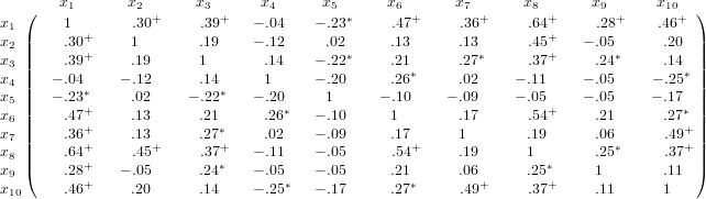
As an empirical illustration of these analytic results, we examine previously unpublished pilot data collected during the dissertation research of Goldstein (1997). These data come from a study that uses the well-known “German Cities” experimental stimuli. These stimuli were used by Goldstein and Gigerenzer (2002) in a series of experiments to empirically validate the recognition heuristic, and in experiments that examined the Take The Best heuristic (Gigerenzer & Goldstein, 1996; Gigerenzer, et al., 1999). These data (Goldstein, 1997) consist of recognition counts from 25 subjects who were asked to indicate whether or not they recognized each of the 83 cities based on their names alone. Each city was assigned a recognition score based on the number of subjects (out of a possible 25) who recognized it. In addition, we have nine binary attributes for each city that serve as predictors — see Table 1 for a description of the predictor cues (Gigerenzer et al., 1999). The inter-correlation matrix of the 10 predictors is presented in Table 2.
The data in Table 2 strongly resemble the optimality conditions described in Conditions 1 and 2. Recognition is significantly and positively correlated with 7 of the 9 predictor cue variables at p<.01. Twenty four of (9 × 8 /2 = ) 36 cue inter-correlations are not significantly greater than 0, which strongly resembles Condition 2. Each of the nine predictors in the array (x2, x3, …, x10) has its highest correlation with recognition with one or two exceptions in each column, i.e., r1j > rkj, ∀ k ∈ {2, 3, …, 10} holds for 7 of the 9 predictors with at most one exception each. The average correlation of the recognition variable with the other nine cue predictors is .29 and the average inter-correlation of the 9 predictors is .11.
To summarize, these data are consistent with the structure of Conditions 1 and 2. The nine predictor cues for the cities appear to contribute “unique” pieces of information to the linear model (8), yet most of these predictors have large positive correlations with recognition. We conclude that in the case of the “German Cities” stimuli, it is an optimal mini-max strategy to “overweight” recognition.
We presented a condition on the predictor cue inter-correlation matrix under which it is optimal to over-weight a single-variable within a linear model, to optimize risk. We demonstrated when this over-weighting condition occurs (Result 1) and what the optimal weighting scheme is (Result 2). To summarize, when a single cue correlates with the other predictors more than they inter-correlated with each other, it is a mini-max strategy, with respect to risk, to over-weight the single cue. We applied these results to a prominent single-variable decision heuristic — the Recognition Heuristic (Goldstein & Gigerenzer, 2002) — and provided a condition where a DM using solely recognition to choose between two choice alternatives would incur precisely the same maximal risk as a decision maker using only knowledge (Result 3). We illustrated these results by analyzing the inter-cue correlation matrix from an experiment using the well-known “German Cities” stimuli. This dataset provides empirical support for the descriptive accuracy of Conditions 1 and 2, and therefore for the over-weighting of a single predictor cue.
The performance of single-variable decision heuristics like the RH depends upon the complex interplay of a DM’s cognitive capacities and the structure of the environment, i.e., the relationships among predictor cues and the criterion variable. When all predictor cues are highly positively correlated we have conditions for a “flat maximum effect”; here a single-variable decision rule will do as well as any other simple weighting rule. In other words, any choice of weighting scheme utilizes, essentially, the same information in the environment. The DM benefits in such “single-factor” environments as he can use a less cognitively demanding strategy and not suffer any serious penalties for doing so. In such single-factor environments the optimal weighting scheme may not resemble a single-variable rule, but the differences in performance are so small that it doesn’t really matter. The DM is “rational” because he/she is balancing cognitive effort with the demands of the environment, the “twin-blades” of Simon’s scissors (Simon, 1990) or seeking to optimize the accuracy / effort tradeoff (Payne et al., 1993).
This article provides a new perspective on the “rationality” of single-variable rules such as the RH. The conditions we have identified are quite different than the conditions previously identified as favorable for single-variable rules, e.g., all predictor cues highly positively correlated. Surprisingly, the over-weighting effect becomes stronger as the inter-correlations in the predictor array become lower, peaking when the predictor cues are mutually uncorrelated. A decision maker employing a single-variable decision heuristic in this environment is “rational” in the sense that he/she is using a decision strategy that is not cognitively demanding and one that resembles an optimal strategy in terms of minimizing risk.
To clarify, we are not proposing a decision heuristic, e.g., pick the most highly correlated predictor cue, but point out that in certain decision environments single-variable heuristics are almost optimal. Our definition of risk, a common benchmark in the statistical literature, may help explain why our “favorable” conditions for a single-variable rule differ from previous ones. Minimizing maximal risk is equivalent to choosing a weighting scheme that is, on average, closest to the true state of the nature, β. This definition accounts for an infinity of possible relationships between the predictor cues and the criterion variable, focusing on the conditions that yield the least favorable relationships. By this measure, it is better to over-weight a single variable that contains some information about all of the predictor cues than to weight, say equally, all of the predictor cues taking the chance that some combination of them may not be at all predictive of the criterion. In this way, we account for an infinity of possible validity structures, even though our formulation does not require any specific assumptions on the validities themselves.
To solve for minimax risk, we only need to know the predictor (cue) inter-correlation matrix and identify the choice of weighting vector a. With minimal assumptions, this is tantamount to assuming a correlational structure on the predictor cues and deciding on a decision heuristic. As a result, we do not assume that the DM has knowledge of the individual validities nor that he/she has an ability to estimate them, in contrast to the lexicographic single-variable heuristic Take The Best (e.g., Gigerenzer et al, 1999). We do assume in our analysis that the decision maker always utilizes the single predictor that conforms to our sufficient conditions. We do not assume any other structure to predictor cue selection or application. Thus, recognition is a natural application of these results, as the Recognition Heuristic does not presuppose a predictor cue selection process.
Our results easily extend to recent generalizations of the RH. Several studies have extended the application of the RH beyond simple 2-alternative forced choice to n-alternative forced choice (Beaman, McCloy, & Smith, 2006; Frosch, Beaman, & McCloy, 2007; McCloy & Beaman, 2004; McCloy, Beaman, & Goddard, 2006); see also Marewski, Gaissmaier, Schooler, Goldstein, & Gigerenzer (2010) for a related framework employing “consideration sets”. Our linear modeling framework does not depend upon the number of choice alternatives being considered. Our only assumption is that the DM differentially selects alternatives based on the value of the criterion as implied by his/her choice of predictor cue weights. Thus, moving from 2 to n alternatives under consideration does not change our key results, a DM utilizing our optimal weighting scheme to select among a set of alternatives will “on average” perform better than another DM using a sub-optimal weighting scheme. Our framework also allows the predictors to be either binary or continuous or any combination thereof. In this way, our results easily extend to continuous representations of recognition. Several authors have previously explored continuous representations of recognition within the contexts of both signal detection models (Pleskac, 2007) and the ACT-R framework (Schooler & Hertwig, 2005).
Although we applied our model successfully in the context of RH, we must remain silent on the psychological nature of some key concepts underlying the theory in this domain. For example, we treat this p-many predictor cue “knowledge” array as an abstract quantity and subsequently do not place any special psychological restrictions or assumptions upon these predictor cues. We also recognize that there is an ongoing debate in the literature as to the interplay between knowledge, learning, and memory with regard to recognition and that there are many factors that influence whether DMs’ choices are consistent with the RH (e.g., Newell & Fernandez, 2006; Pachur, Bröder, & Marewski, 2008; Pachur & Hertwig, 2006). However, our model is mute with respect to these debates.
The results we have presented are general, and while we have restricted their application to the study of recognition, they could be applied to other domains. For example, in a well-publicized study on heart disease, Batty, Deary, Benzeval, and Der (2010) found that IQ was a better predictor of heart disease than many other, more traditional, predictors such as: income, blood pressure, and low physical activity. One possible explanation of their findings is that, historically, IQ tends to correlate to some degree with each of the remaining predictors (e.g., Batty, Deary, Schoon, & Gale, 2007; Ceci & Williams, 1997; Knecht et al., 2008). In light of the results presented in our paper, it is perhaps not so surprising that IQ is a “robust” predictor of heart disease.
Our results do not imply that ordinary least squares or other statistical/machine-learning weighting processes are “sub-optimal.” Given an infinite amount of data, weighting schemes derived from such processes would indeed be optimal with respect to almost any measure. Our results apply to fixed weighting schemes, which, in the context of small sample sizes tend to perform very well as they do not “over-fit” the observed data. In other words, fixed weighting schemes cross-validate extremely well compared to other, more computationally intensive, estimation procedures for situations involving small sample sizes and/or large variances in the error terms.
Gigerenezer et al., (1996; 1999) argue that “fast and frugal” heuristics are a rational response to the “bounded” or “finite” computational mind of a decision maker. This article raises many new questions regarding the rationality of simple decision heuristics. Given infinite computational might and a relatively small sample of data, a “Laplacean Demon’s” choice of weighting scheme might resemble that of a “fast and frugal” decision maker. In other words, DMs could be reasoning like a “Laplacean Demon” would if the demon were given limited information, but retained the assumption of infinite computational ability.
Batty, G. D., Deary, I. J., Benzeval, M., & Der, G. (2010). Does IQ predict cardiovascular disease mortality as strongly as established risk factors? Comparison of effect estimates using the West of Scotland Twenty-07 cohort study. European Journal of Cardiovascular Prevention and Rehabilitation, 17, 24–27.
Batty, G. D., Deary, I. J., Schoon, I., & Gale, C. R. (2007). Childhood mental ability in relation to food intake and physical activity in adulthood: The 1970 British cohort study. Pediatrics, 119, 38–45.
Baucells, M., Carrasco, J. A., & Hogarth, R. M. (2008). Cumulative dominance and heuristic performance in binary multiattribute choice. Operations Research, 56, 1289–1304.
Beaman, C. P., McCloy, R., & Smith, P. T. (2006). When does ignorance make us smart? Additional factors guiding heuristic inference. In R. Sun & N. Miyake (Eds.), Proceedings of the Twenty-Eighth Annual Conference of the Cognitive Science Society. Hillsdale, NJ: Lawrence Erlbaum Associates.
Bröder, A. (2000). Assessing the empirical validity of the “take-the-best” heuristic as a model of human probabilistic inference. Journal of Experimental Psychology: Learning, Memory, and Cognition, 26, 1332–1346.
Bröder, A., & Schiffer, S. (2003). Take the best versus simultaneous feature matching: Probabilistic inferences from memory and effects of representation format. Journal of Experimental Psychology: General, 132, 277–293.
Brunswik, E. (1952). The conceptual framework of psychology. Chicago: The University of Chicago Press.
Ceci, S. J., & Williams, W. M. (1997). Schooling, intelligence, and income. American Psychologist, 52, 1051–1058.
Davis-Stober, C. P., Dana, J., & Budescu, D. V. (2010) A constrained linear estimator for multiple regression. Psychometrika, in press.
Dawes, R. M. (1979). The robust beauty of improper linear models. The American Psychologist, 34, 571–582.
Dawes, R. M., & Corrigan, B. (1974). Linear models in decision making. Psychological Bulletin, 81, 95–106.
Einhorn, H. J., & Hogarth, R. M. (1975). Unit weighting schemes for decision making. Organizational Behavior and Human Performance, 13, 171–192.
Fasolo, B., McClelland, G. H., & Todd, P. M. (2007). Escaping the tyranny of choice: When fewer attributes make choice easier. Marketing Theory, 7, 13–26.
Frosch, C. A., Beaman, C. P., & McCloy, R. (2007). A little learning is a dangerous thing: An experimental demonstration of ignorance-driven inference. The Quarterly Journal of Experimental Psychology, 60, 1329–1336.
Gigerenzer, G., & Goldstein, D. G. (1996). Reasoning the fast and frugal way: Models of bounded rationality. Psychological Review, 103, 650–669.
Gigerenzer, G., Todd, P. M. & the ABC Research Group. (1999). Simple heuristics that make us smart. New York: Oxford university Press.
Goldstein, D. G. (1997). Models of bounded rationality for inference. Doctoral thesis, The University of Chicago. Dissertation Abstracts International, 58(01), 435B. (University Microfilms No. AAT 9720040).
Goldstein, D. G., & Gigerenzer, G. (2002). Models of ecological rationality: The recognition heuristic. Psychological Review, 109, 75–90.
Hammond, K. R., Hursch, C. J., & Todd, F. J. (1964). Analyzing the components of clinical inference. Psychological Review, 71, 438–456.
Hertwig, R., & Todd, P. M. (2003). More is not always better: The benefits of cognitive limits. In D. Hardman, & L. Macchi (Eds.), Thinking: Psychological perspectives on reasoning, judgment and decision making (pp. 213–231). Chichester, England: Wiley.
Hogarth, R. M., & Karelaia, N. (2005). Ignoring information in binary choice with continuous variables: When is less “more”? Journal of Mathematical Psychology, 49, 115–124.
Hogarth, R. M., & Karelaia, N. (2006). “Take-The-Best” and other simple strategies: Why and when they work “well” with binary cues. Theory and Decision, 61, 205–249.
Katsikopoulos, K. V., & Martignon, L. (2006). Naïve heuristics for paired comparisons: Some results on their relative accuracy. Journal of Mathematical Psychology, 50, 488–494.
Keeney, R. L., & Raiffa, H. (1993). Decisions with multiple objectives: Preferences and value tradeoffs. Cambridge: Cambridge University Press.
Knecht, S., Wersching, H., Lohmann, H., Bruchmann, M., Duning, T., Dziewas, R., Berger, K., & Ringelstein, E. B. (2008). High-normal blood pressure is associated with poor cognitive performance. Hypertension, 51, 663–668.
Marewski, J. N., Gaissmaier, W., Schooler, L. J., Goldstein, D. G., & Gigerenzer, G. (2010). From recognition to decisions: Extending and testing recognition-based models for multi-alternative inference. Psychonomic Bulletin & Review, 17, 287–309.
Martignon, L., & Hoffrage, U. (1999). Why does one-reason decision making work? A case study in ecological rationality. In G. Gigerenzer, P. M. Todd, & the ABC Research Group (Eds.), Simple heuristics that make us smart (pp. 119–140). New York: Oxford University Press.
Martignon, L., & Hoffrage, U. (2002). Fast, frugal, and fit: Simple heuristics for paired comparison. Theory and Decision, 52, 29–71.
McCloy, R., & Beaman, C. P. (2004). The recognition heuristic: Fast and frugal but not as simple as it seems. In K. Forbus, D. Gentner, & T. Regier (Eds.), Proceedings of the Twenty-Sixth Annual Conference of the Cognitive Science Society (pp. 933–937). Mahwah, NJ: Lawrence Erlbaum Associates.
McCloy, R., Beaman, C. P., & Goddard, K. (2006). Rich and famous: Recognition-based judgment in the Sunday Times rich list. In R. Sun & N. Miyake (Eds.), Proceedings of the Twenty-Eighth Annual Conference of the Cognitive Science Society (pp. 1801–1805). Hillsdale, NJ: Lawrence Erlbaum Associates.
Newell, B. R., & Fernandez, D. (2006). On the binary quality of recognition and the inconsequentiality of further knowledge: Two critical tests of the recognition heuristic. Journal of Behavioral Decision Making, 19, 333–346.
Newell, B. R., & Shanks, D. R. (2003). Take the best or look at the rest? Factors influencing “one-reason” decision making. Journal of Experimental Psychology: Learning, Memory, and Cognition, 29, 53–65.
Pachur, T., & Biele, G. (2007). Forecasting from ignorance: The use and usefulness of recognition in lay predictions of sports events. Acta Psychologica, 125, 99–116.
Pachur, T., Bröder, A., & Marewski, J. N. (2008). The recognition heuristic in memory-based inference: Is recognition a non-compensatory cue? Journal of Behavioral Decision Making, 21, 183–210.
Pachur, T., & Hertwig, R. (2006). On the psychology of the recognition heuristic: Retrieval primacy as a key determinant of its use. Journal of Experimental Psychology, 32, 983–1002.
Payne, J. W., Bettman, J. R., & Johnson, E. J. (1993). The adaptive decision maker. New York: Cambridge University Press.
Pleskac, T. J. (2007). A signal detection analysis of the recognition heuristic. Psychonomic Bulletin & Review, 14, 379–391.
Scheibehenne, B., & Bröder, A. (2007). Predicting Wimbledon 2005 tennis results by mere player name recognition. International Journal of Forecasting, 23, 415–426.
Schooler, L. J., & Hertwig, R. (2005). How forgetting aids heuristic inference. Psychological Review, 112, 610–628.
Serwe, S., & Frings, C. (2006). Who will win Wimbledon? The recognition heuristic in predicting sports events. Journal of Behavioral Decision Making, 19, 321–332.
Shanteau, J., & Thomas, R. P. (2000). Fast and frugal heuristics: What about unfriendly environments? Behavioral and Brain Sciences, 23, 762–763.
Simon, H. A. (1990). Invariants of human behavior. Annual Review of Psychology, 41, 1–19.
Snook, B., & Cullen, R. M. (2006). Recognizing national hockey league greatness with an ignorance-based heuristic. Canadian Journal of Experimental Psychology, 60, 33–43.
Todd, P. M. (1999). Simple inference heuristics versus complex decision machines. Minds and Machines, 9, 461–477.
Wainer, H. (1976). Estimating coefficients in linear models: It don’t make no nevermind. Psychological Bulletin, 83, 213–217.
This document was translated from LATEX by HEVEA.