Judgment and Decision Making, vol. 5, no. 4, July 2010, pp.
258-271
Less-is-more effects without the recognition heuristicC. Philip Beaman* 1,2, Philip T. Smith1,
Caren A. Frosch1, 3 and Rachel McCloy1, 4
1 School of Psychology & Clinical Language Sciences,
University of Reading
2 Centre for Integrative Neuroscience & Neurodynamics,
University of Reading
3 Department of Psychology, Queen’s University,
Belfast
4 Government Social Research Unit, HM Treasury |
Inferences consistent with “recognition-based” decision-making may
be drawn for various reasons other than recognition alone. We
demonstrate that, for 2-alternative forced-choice decision tasks,
less-is-more effects (reduced performance with additional learning)
are not restricted to recognition-based inference but can also be seen
in circumstances where inference is knowledge-based but item knowledge
is limited. One reason why such effects may not be observed more
widely is the dependence of the effect on specific values for the
validity of recognition and knowledge cues. We show that both
recognition and knowledge validity may vary as a function of the
number of items recognized. The implications of these findings for the
special nature of recognition information, and for the investigation
of recognition-based inference, are discussed.
Keywords: less-is-more effect, fast and frugal judgment.
1 Introduction
Investigations of the recognition heuristic (RH) typically involve
participants making judgments about items about which they have limited
knowledge, such as the relative sizes of cities in the USA. For
example, a participant might be presented with the two cities
San Diego and San Antonio and asked which is bigger.
In the classic work of Goldstein and Gigerenzer (2002), it is assumed
that the participant will guess if they recognize neither of the items,
they will use whatever additional knowledge is available to make a
decision if they recognize both of the items and, crucially, if they
recognize only one of the items, they will choose this item as the
larger without consulting any other cues or searching for further
information (the Recognition Heuristic or RH). This
is because items of larger size are more likely to be encountered,
hence more likely to be recognized (the recognition-magnitude
correlation). Recognizing one of the two items is thus a useful cue for
choosing the recognized item. If both items are recognized, however,
additional knowledge is needed to make the decision and such additional
knowledge may be very limited. Recognition-driven inference can give
rise to the less-is-more effect (LiME), whereby individuals
who recognize many of the items often perform worse than individuals
who recognize fewer of the items (Goldstein & Gigerenzer, 2002).
The LiME is a counter-intuitive finding, predicted to occur under
given circumstances if the RH is applied (Goldstein & Gigerenzer,
2002; McCloy, Beaman & Smith, 2008). The counter-intuitive nature of
the LiME prediction allows for a strong test of the RH and has been
used as a rhetoric device to promote the heuristic (Borges, Goldstein,
Ortmann & Gigerenzer, 1999; Gigerenzer, 2007; Schooler & Hertwig,
2005). Evidence for the LiME has also been observed empirically
(Frosch, Beaman & McCloy, 2007; Goldstein & Gigerenzer, 2002; Reimer
& Katsikopoulos, 2004) but, counter to this, failures to observe the
effect have also been cited in attempts to refute the RH (e.g., Boyd,
2001; Dougherty, Franco-Watkins & Thomas, 2008; Pohl, 2006). At least
as originally introduced, a LiME is a mathematical necessity (given
certain assumptions) rather than a proof of recognition-based
inference. Nevertheless, the consensus appears to be that the
observation of a LiME implies that the recognition heuristic was
employed (Pachur, Mata & Schooler, 2009), and that the use of
knowledge will dilute or reduce the size of the LiME (e.g., Hilbig,
Erdfelder & Pohl, 2010). Here we explore whether LiMEs are also
mathematical necessities if those assumptions are altered somewhat —
specifically if inference is no longer recognition-based but instead
makes reference to some form of knowledge.
LiMEs need not appear only when the RH is studied in isolation. They are
also predicted by formal models of knowledge-based inference if those models
exploit the recognition principle. Gigerenzer and Goldstein (1996) used
the appearance of the effect as part of their comparison of five
integration algorithms with the Take The Best (TTB) algorithm
(Gigerenzer & Goldstein, 1996; pp. 656–661). TTB and all of the
integration algorithms were implemented such that, in each case,
recognition was used as a cue if only one item was recognized (p. 657).
Unsurprisingly, all six algorithms produced a non-monotonic
relationship between recognition and correct inference (Gigerenzer &
Goldstein, 1996, Figure 6). However, as we will demonstrate, LiMEs can
be produced by knowledge-based decision-making processes which use
neither recognition-driven inference nor the related
speed-of-retrieval inference that Schooler and Hertwig (2005) have
shown produces similar advantageous effects for moderate over lesser
forgetting rates. The first aim of this paper is to prove by analytical
means that LiMEs can be produced by knowledge-based decision-rules.
They are not unique to recognition-driven inference and cannot
therefore be viewed as providing unconditional support for this
hypothesis. Our second aim is to examine, using the basic framework
developed, how both recognition and knowledge validities vary as a
function both of the correlation between recognition and magnitude and
the number of items recognized.
1.1 Moderators of the recognition-magnitude correlation.
In Goldstein and Gigerenzer’s original (2002) formulation of the RH,
additional knowledge is used only as a tie-breaker to decide between
two recognized items. When a single item is recognized, inference is
purely recognition-driven. This aspect has aroused much interest and
has proven controversial (Gigerenzer & Brighton, 2009; Hilbig &
Pohl, 2008; Hilbig, Pohl & Bröder, 2009; Newell & Fernandez, 2006;
Newell & Shanks 2004; Pachur & Hertwig, 2006; Pachur, Bröder &
Marewski, 2008; Pohl, 2006; Richter & Späth, 2006). In an
alternative formulation, limited knowledge can be used even when only
one item is recognized. This alternative formulation is worth
examining because a number of accounts, generally favorable to the
RH, have seemingly relaxed the criteria for its application. For
example, Volz et al. (2006, p. 1935) conclude, on the basis of
neuroimaging evidence that, “the processes underlying RH-based
decisions go beyond simply choosing the recognized
alternative.” Additionally, the discrimination index proposed by
Hilbig and Pohl (2008) led them to conclude that a substantial number
of recognition-consistent choices were informed by further information
other than recognition alone.
The relationship (whether positive or negative) between the
recognition of an item and its magnitude is clearly central to the
RH. It works because, in the tasks to which this approach has been
successfully applied, larger items are more prominent (more
newsworthy, more important, etc.) than smaller items and this leads to
larger items being more likely to be recognized. However, if the
question related to the relative size of pairs of birds and the single
recognized item was a house-sparrow, the Recognized →
Larger inference makes much less sense than when the same options are
presented but the question relates to the relative population size of
the two birds.1 This
highlights the fact that recognition actually correlates with
prominence, which may not itself correlate with all forms of magnitude
per se. The prominence-recognition correlation also may not
hold — or at least, it may vary in size — if the items experienced
as prominent vary between individuals. One potential moderating factor
is sampling bias. The newspaper example given by Goldstein and
Gigerenzer (2002) is a good case. In this example, it is suggested
that a city may be recognized if it is frequently mentioned in a
newspaper, and that a larger city is more likely to be so
mentioned. The individual receiving the newspaper is implicitly
assumed to be a fairly passive processor of the information contained
within the newspaper. No consideration is given to the potential
difference between an individual who actively seeks out a newspaper
and one who does not, or to potential differences between choice of
reading matter. These may have very different content (e.g., the
New York Review of Books versus the National
Enquirer), and each of which might be sought out, or passively
encountered, to different degrees by different individuals or groups
of individuals. Calculating the recognizability of a city from the
relative frequency with which it is mentioned in any one publication
may be misleading if applied to a group of individuals who
disproportionately sample from another publication or from different
sections of the same publication (e.g., the sporting pages versus the
“style” section). Overall, biased sampling of this type may be good
or bad for the performance of the heuristic, depending on whether a
disproportionate number of “large” items are sampled, which would
enhance the validity of recognition (e.g., a soccer fan will recognize
more towns with premier league soccer teams) or whether sufficient
“small” items are sampled to reduce the magnitude-recognition
correlation (e.g., a golf fan will recognize more towns with famous
golf courses, but such towns do not on the whole tend to be large in
size).
A basic premise in what follows is that, for any given individual, there
are several subgroups of items which the individual is able to
recognize and about which they may also have partial knowledge. This is
particularly likely if they are local to the individual in some way or
if they form part of a set of items of special interest to that
individual. For example, the third author has observed anecdotally that
the only German citizens of her acquaintance who reliably recognize the
Yorkshire city of Leeds are football fans. Coincidentally, British
citizens of her acquaintance show the same pattern for the
Nordrhein-Westfalen city of Leverkusen. Hence, anecdotally at least, it
appears that football fans and those uninterested in the game may have
differential access to subsets of European cities. Special access to
information regarding subgroups may also vary with the choice domain, a
point which is easily confirmed using existing empirical data. For
example, by-item analysis of data taken from an experiment by McCloy,
Beaman, Frosch and Goddard (2010), in which a group of 40
participants were asked to indicate which of a group of famous
individuals they recognized, found no significant effect of the gender of the
participant on the overall recognition rate, F(1, 43) = 2.3,
p = .14 but a significant effect of the reasons why the
individuals rose to fame (as either sports personalities, fashion and
show-business professionals, rock stars or business people),
F(3, 43) = 13.48, p < .001, and a
significant interaction between this factor and the gender of the
participant, F(3, 43) = 13.44, p < .001.
Males recognized, on average, sports personalities 78% of the time
(females = 55%) and rock stars 75% of the time (females = 66%). In
contrast, females recognized fashion and show-business professionals
57% of the time (males = 33%) and the two genders were both poor at
recognizing business people, males = 16%, females = 11%. Thus, gender
is a factor which provides, or at least contributes to, differential
access to different subsets of rich and famous people. In what follows,
we consider similar situations where, for an individual within the
environment, there is no simple correlation between recognition and
magnitude because subsets of the items are prominent for reasons
unconnected to magnitude (e.g., the age, gender or special interests of
the individual).
2 Study 1: Models predicting the LiME
To formally examine the appearance of LiMEs, we suppose a pool of N
items, split into several subsets A, B, C, …. Within each
subset the participant is able to recognize u v, w, …items,
respectively. In a typical test of recognition-driven inference, the
experimenter selects items quasi-randomly from the pool. Since the
constraints on the experimenter are unknown, a random selection from
N is assumed. In the basic case, pairs of items are chosen, and the
participant’s task is to say which is larger. For purposes of
exposition, we restrict attention to situations with just three
subsets. The models can easily be extended to other cases (e.g., the
participant is asked to choose between more than two items [Frosch et
al., 2007; McCloy et al., 2008] and/or the pool is split into more
than three subsets).
2.1 The basic framework
Suppose that, when presented with a two-alternative forced choice
task, an individual recognizes from among the two alternatives i
items from subset A, j items from subset B, and k items from
subset C. On a given trial, only two items are presented, so i,
j, k range from 0 to 2, with i + j + k ≤ 2. That is, the
number of items recognized on any trial could vary from 0–2 for any
of the three subsets but the total number recognized obviously cannot
exceed the two items presented. pijk is the probability that this
event occurs. (For example, if i=1, j=1, and k=0, pijk is
the probability of recognizing one item from subset A and one from
subset B.) pijk is obviously dependent on how many items the
participant can recognize in each of the subsets, but is independent
of the decision rule adopted. αijk is the probability of
success, given the recognition of i, j and k items from their
respective subsets. This parameter is dependent on the decision rule
the participant adopts and is the only thing that distinguishes the
models we consider. The overall probability of success P(u,v,w) is
given by:
|
P(u,v,w) = Σijk αijk pijk
(1) |
Having outlined the basic framework, we can present the models. The RH
model requires little introduction, the alternative against which it
is to be compared we refer to as LINDA (Limited INformation and
Differential Access).
2.1.1 The Recognition Heuristic (RH) model
The distinguishing feature of the RH model is that the participant
chooses the recognized item when only one item is recognized. So
α000 = 0.5 (no item recognized, pure guess); α100,
α010, and α001 reflect the success of the
recognition heuristic (they should be greater than chance if the
recognition heuristic has some validity, and should be quite large for
the clearest LiMEs); α110, α101, α011,
α200, α020, α002 reflect use of
knowledge (two items are recognized, so additional knowledge is used
to discriminate them; LiMEs should be clearest if these knowledge
probabilities are close to chance).
2.1.2 The Limited INformation and Differential Availability (LINDA)
model
As the name implies, this model requires two basic assumptions:
-
The limited information assumption. For each recognized
item, the individual has relevant but limited information about its
size (e.g. that the size is above the population median). For the
sake of simplicity, this is presented as if it were criterion-based
knowledge rather than inference from cues. However, recent data show
little impact on the use (or non-use) of recognition-based inference
when criterion knowledge is available (Hilbig et al.,
2009). Reanalysis of data by Hilbig et al. (2009) also shows that
— at least for the domain they examined (the size of cities in
Belgium) — participants showed something approximating median
knowledge. Hilbig et al. recorded participants’ estimates of the
populations of each of the cities they were asked to consider so it
is possible to calculate, per participant, the probability that they
correctly judged whether the city in question was above or below the
sample median.2 This information may not be totally reliable, and we
use parameters pA, pB, … for the probabilities that
information regarding a recognized item belonging to subsets A,
B, … is accurate. From Hilbig et al.’s data, participants
were judging an item to be the correct side of the sample median on
69% of occasions on average (s.d. = 13%). In what follows, for the
most part, we assume pA = pB = pC = 1 as this is the simplest
case but varying this parameter (for example changing it from 1 to
.7, or 70% of cases correct) only alters the magnitude of the
effects observed and does not affect the general conclusions.
- The differential availability assumption. Some subsets
are more accessible than others so that, for a given individual,
more items may be recognizable within one subset than within
another. Note that this assumption does not necessarily imply no
correlation between magnitude and recognition, but it allows the
extent of this correlation to be manipulated by varying the relative
recognizability of the subsets.
The limited information assumption assumes that there is, at the least,
some information available at the time of decision-making against which
to evaluate the usefulness of choosing the recognized item in any given
case. The reliability of this information may also vary. Either the
information may be incorrect or (potentially) it may be misapplied in
some way. For simplicity, these possibilities are both reflected in the
value of a single parameter, as noted in assumption 1. The differential
availability assumption states merely that, within any set, the items
within some subsets are more or less recognizable than the items within
some other subset.
2.1.3 Numerical example
| Figure 1: Proportion correct using LINDA and the RH for different
orderings of subsets (and hence different recognition-magnitude
correlations). ABC ordering is equivalent to a
recognition-magnitude correlation of ρ = .919 and ACB
ordering is equivalent to ρ = .306. |
For the LINDA model described above, consider the situation where
individuals have what we will term median knowledge of items
from pool N, i.e. they accurately know whether each
recognized item is above or below median. Subset A includes items in
the top quartile of the size distribution, subset B includes items
in the second highest quartile of the size distribution, and subset
C contains all the remaining items. The Appendix gives the
derivations of explicit expressions for all the terms in Equation (1).
In the first example, it is assumed for purposes of exposition that
median knowledge is perfect, i.e., that the median knowledge about a
recognized item is accurate with no chance of error (pA = pB =
pC = 1). This assumption is relaxed in later examples.
In order to formally compare the RH model with the LINDA model, the
models are designed to perform equally well when all items are
recognized. In the current simple example, where all items are
recognized, u and v are the number of items recognized from
subsets A and B, which constitute the top two quartiles of the
distribution, respectively, and w is the number of remaining
recognized items (subset C), so if u=v=25 and w=50, the total
number recognized, then n=N=100. The probabilities of a correct
inference when recognizing 2 items in any of the possible combinations
that may occur (e.g., 2 from u, or 1 from u and 1 from v, and so
on) are given by the equations presented in sections 1 and 3 of the
Appendix. LINDA’s performance with full recognition is the sum of
these probabilities, which works out as 0.7525, so in the RH model
probabilities of success when both presented items are recognized were
also set to 0.7525. The size of the pool from which the test items are
drawn is set at 100 but the same pattern of results is obtained for
all large values of N. The key prediction is the relation between
the proportion of correct decisions (P in equation (1)) and n, the
number of items in the pool the participant can recognize.
To examine how these models interact with the recognition of items from
different subsets, consider the cases where there is a close link
between the recognition of items and the subsets from which they are
drawn. The notation ABC means that items from subset
A are all more recognizable than the items from subset
B, which in turn are all more recognizable than the items from
subset C. This strict ordering of recognition is obviously
unrealistic but is useful to demonstrate relations between recognition
and the properties of the two models and could easily be relaxed to
allow some overlap between the recognition of items from different
subsets. If this constraint is enforced, and the equations given in the
Appendix calculated accordingly, then the results shown in Figure 1 are
obtained.
Figure 1 shows the performance of LINDA and the RH model for two
different magnitude-recognition orderings: ABC (items in the top
quartile of the size distribution are most recognizable and items below
median are least recognizable) and ACB (items in the top quartile are
most recognizable, then items from below the median and finally items
from the second quartile). ABC ordering corresponds to a strong
magnitude-recognition correlation (ρ = .919) and ACB ordering to
a smaller, but still positive, correlation between magnitude and
recognition (ρ = .306). The plausibility of such an ordering of
recognition might be queried, but it is fairly easy to generate
scenarios in which particularly large items are most recognizable, then
particularly small items. For cities, as already mentioned, the
possession of a good golf course enhances its recognizability (in the
UK: Carnoustie, Lytham St Annes, St Andrews, Sunningdale, Turnberry)
but good golf courses are not, for the most part, associated with large
cities because of the space they require. The ABC ordering produces
effects we would expect from the literature. The RH model, using the
recognition heuristic, shows the expected LiME, while the
knowledge-based LINDA model shows a monotonic relation between
proportion correct and number of recognizable items.
| Figure 2: Proportion correct for the LINDA model when discrimination
between two recognized items is at chance. The same calculations can be
made for the RH but are not given here. A spreadsheet to simulate the
RH was produced by McCloy et al. (2008) and can be used for calculating
the RH’s predictions for situations corresponding to
those in this Figure depicted for LINDA. The spreadsheet is available
to download from
http://www.personal.rdg.ac.uk/~sxs98cpb/philip_beaman.htm although
note the calculations in this spreadsheet assume automatic application
of the RH, even when recognition is not a good cue. |
The situation is quite different for the ACB ordering: here it is
LINDA that produces an inverted-U shaped function and a LiME. LiMEs
therefore cannot necessarily imply use of the recognition heuristic
— even given a positive magnitude-recognition correlation — but
may occur for other reasons. The inverted-U shaped functions that
characterize the LiME indicate that a task becomes more difficult once
the number of recognizable items passes a certain level. In the case
of the RH model and the ABC ordering, this is because “easy”
decisions (select the recognized item when only one item is
recognized) are gradually outnumbered by “difficult” decisions
(choose between items, both of which have been recognized) as the
number of recognizable items increases. In the case of LINDA and the
ACB ordering, moderate levels of recognition produce many easy
decisions (discriminating a recognized item drawn from subset A from a
recognized item drawn from subset C) but the decisions become more
difficult when items of intermediate size, from subset B, begin to
join the pool of recognizable items as the number of recognizable
items increases. If the size of the LiME is defined as the maximum
proportion correct minus the proportion correct when n = N (e.g.,
McCloy et al., 2008) then the effect size for the RH and for LINDA is
similar when LINDA has totally reliable information (for ordering ABC,
RH effect size = .06, for ordering ACB, LINDA effect size = .06). The
size of the effect is reduced if LINDA’s information is less reliable
(e.g., if pA = pB = pC = 0.7, effect size for ordering ACB =
.03) but increases if the assumption is made that LINDA has difficulty
with discriminations when both items are recognized.
In calculating LINDA’s predictions, we previously
assumed no extra difficulty was involved in having to choose between
two recognized items, but this assumption might not be realistic: choosing between
two recognized items may, in some instances, be extremely difficult. An
extreme version of this is shown in Figure 2. Here it is assumed that
LINDA makes decisions in the way already outlined when only one item is
recognized, but does not have the capacity to make a decision when both
items are recognized, and so is obliged to guess. The situation
resembles one outlined in Goldstein and Gigerenzer (2002, pp. 84–85) in
which German participants were experimentally exposed to the names of
US cities without being presented with any further information which
might be of use, and is also comparable to Schooler and
Hertwig’s (2005) ACT-R implementation of the
recognition heuristic, which also assumed chance level performance when
both items were recognized (Schooler & Hertwig, 2005, p. 614).
Figure 2 shows clear LiMEs also appear for this version of LINDA.
Interestingly, unlike the RH model, which requires quite large
magnitude-recognition correlations to allow recognition validity to
exceed knowledge validity, LINDA shows LiMEs for all values of ρ,
although the largest LiMEs occur for the largest values of ρ. No
“recognition validity” parameter was built into LINDA a
priori (although clearly the validity of recognition is to some
extent reflected in the values of ρ ) so these results are not
subject to the criticism that it is trivial to show LiMEs if knowledge
validity is set sufficiently low relative to recognition validity
(McCloy et al., 2008). Once again, then, a knowledge-based decision
model produces LiMEs, and thus — once again – LiMEs are not a
unique prediction of the RH model.
2.2 Discussion
Whilst the RH and LINDA give LiMEs in different circumstances, the
effects are produced for essentially the same reasons. When relatively
few items are recognizable, the task is easier than when many items are
recognizable. In the case of the RH model, when an intermediate number
of items are recognizable the individual is more frequently confronted
with the easy decision of selecting the one item recognized, and this
position is reversed when many items are recognizable. For the LINDA
model, performance for intermediate levels of recognition is good
because the participant is often asked to make the easy discrimination
between an item drawn from top quartile (subset A) and an item
drawn from the bottom quartiles (subset C). Adding items from
the second highest quartile (subset B), makes the task more
difficult and leads to a drop in performance. Natural examples of
highly recognizable subsets comprised of small items (C) are
required to make this analysis plausible. In addition to the examples
of cities with famous golf courses already mentioned, there are
numerous remote towns famous for being inaccessible (and therefore
necessarily small): Alice Springs, Lerwick, Machu Picchu and
Spitzbergen, and in other domains, e.g., the population sizes of
various animal species, there are animals famous for being endangered
(e.g., Giant Panda, Gorilla) which are more immediately recognizable
than animal species with sustainable but by no means large populations.
The fluency rule, discussed by Schooler and Hertwig (2005), also
produces similar results to LINDA and, once again, for similar
reasons. In the context of the fluency rule, the “less” of
less-is-more refers to forgetting rates rather than recognition rates
as in the RH. In that case, intermediate rates of decay allow for
better discrimination between items than low rates of decay (items
retrieved more quickly are presumed to be larger). This leads to the
only other “knowledge” based LiME of which we are aware. Crucially,
however, the fluency rule does not use or require further knowledge
beyond the fact of fast retrieval. Thus, although it produces LiMEs of
a kind, these are arguably recognition rather than
knowledge-driven. Knowledge about the item itself is never consulted,
only knowledge pertaining to the act of retrieval or recognition.
Regardless of the validity of this argument, our results nevertheless
suggest that LiMEs might be both more prevalent, and more difficult to
ascribe to a single strategy, than previously assumed. LINDA
demonstrates that LiMEs can occur for knowledge-based decisions and
also that, when discrimination between two recognized items is
sufficiently difficult, these effects can occur regardless of the
recognition-magnitude correlation.
2.2.1 Reasons for the elusiveness of less-is-more
The above argument seems to imply that LiMEs should be observed
empirically far more readily than seems to be the case. However,
whilst the effect has been empirically verified on some occasions
(Borges, Goldstein, Ortmann, & Gigerenzer, 1999; Frosch et al., 2007;
Goldstein & Gigerenzer, 2002; Reimer & Katsikopoulos, 2004; Snook &
Cullen, 2006) it has not been observed universally (Boyd, 2001; Pachur
& Biele, 2007; Pohl, 2006). One reason for this may be that LiMEs
occur in different situations for different reasons. Whilst it is
possible to find a LiME under circumstances where a LINDA-like
decision-rule might be operating, such an effect would be easier to
discover if the magnitude-recognition correlation was moderate rather
than large, and when the information was particularly reliable, or the
discrimination between two recognized objects particularly difficult
(see Figure 2). Consequently, it would be relatively easy to miss
such an effect if the experimental situation was deliberately designed
to maximize the magnitude-recognition correlation, as many have been
(e.g., Pohl, 2006). There is a clear difference between a model
showing a LiME “in principle” when all factors are under control and
a LiME appearing in a standard experimental design which may be
statistically underpowered to show a small LiME in a noisy
environment. One way around this might be to partition subjects into
groups based upon how much knowledge they appear to employ to inform
nominally “recognition-based” inferences (using e.g., the methods
developed by Hilbig and Pohl (2008) or Hilbig et al. (2009)). It
might then be possible to examine whether the appearance or size of
any LiME is negatively associated with knowledge used (as proponents
of the RH might propose) or if the relation is more complicated (as
LINDA would predict).
A second and more interesting possibility is that insufficient
attention has been paid to some of the parameters that need to be
controlled for a situation to arise where LiMEs would be expected. For
example, the key prerequisite of the LiME produced by the RH is that
recognition validity should exceed knowledge validity. Reliable
manipulation of the recognition and knowledge validity parameters can
be problematic, however. In Goldstein and Gigerenzer’s (2002) account,
it is implicit that both recognition and knowledge validity are, or
can be, independent of n, the number of recognizable items in the
pool of items from which the stimuli are drawn. For example, Figure 2
(p. 79) of their account illustrates the LiME by holding recognition
validity constant and varying knowledge validity and number recognized
independently (between and within hypothetical individuals,
respectively). This is important because n may not be under
experimental control, hence a priori estimates of recognition
and knowledge validities may be misleading. Later in their paper,
Goldstein and Gigerenzer (2002, p. 80) acknowledge that,
“recognition and knowledge validities usually vary when one
individual learns to recognize more and more objects from experience”
but they also appear to endorse the view that, if multiple individuals
are involved, who recognize different numbers of objects, it is
possible that “each individual has roughly the same recognition
validity” (Goldstein & Gigerenzer, p. 80). However, in situations
where the recognition-magnitude correlation is high, an individual who
recognizes only a few items from the pool of items will mostly
recognize very large items. Hence, on any given trial, a recognized
item for that individual is likely to be larger than the unrecognized
item. In contrast, an individual who recognizes more items from the
pool will encounter more trials when the single item they recognize is
not larger than the unrecognized item.
It thus seems a priori unlikely that recognition validity can
be independent of n, where n varies among
individuals. Similarly, when both items are recognized and
individuals are obliged to use their knowledge, an individual who only
recognizes a few items from the pool is likely to encounter items of a
similarly large magnitude when both are recognized. Such items may be
less discriminable than the pairs of items — drawn from a greater
range of sizes — encountered by an individual able to recognize many
items. Hence it also seems a priori unlikely that knowledge
validity can be independent of n.
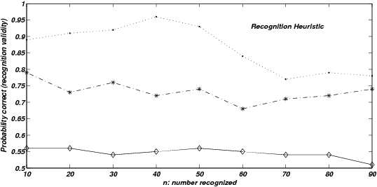
| Figure 3: Probability correct, given only one of two items are
recognized according to recognition (RH) and knowledge-based (LINDA)
models. This is equivalent to Goldstein and
Gigerenzer’s (2002) concept of recognition validity for
the RH model and to the validity of recognition-consistent inference
for the LINDA model. The x-axis only runs from 10–90 items recognized
(out of a possible 100) because the graph plots probability correct
given that exactly one of the two presented items is recognized. |
To formally test the specific question of whether recognition and
knowledge validities can be independent of n, it is possible
to derive values associated with both recognition and knowledge
validity and examine the effect of varying n upon these
values. First, consider recognition validity. Goldstein and Gigerenzer
(2002) present two computer simulations (pp. 80–82) that partially
address this by varying recognition validity varied as a function of
either n (number recognized) or N (the size of the
pool from which the stimuli are taken). Their results, however, are
presented only in terms of overall accuracy (the percentage or
proportion of correct inferences calculated across all choices,
including those informed by knowledge or the result of guesswork)
rather than directly examining the effects upon recognition validity
itself. Using the previously presented notation, the probability of
being correct given that only one of the two presented items is
recognized is as follows:
|
| | α100 p100 + α010 p010 + α001p001 |
|
| p100 +
p010 + p001 |
|
(2) |
The probability expressed in this equation is obviously equivalent to
recognition validity and can be calculated for both LINDA and the RH
model according to the method outlined in the Appendix. Figure 3 shows
recognition probabilities, conditional on recognizing one item of a
stimulus pair (i.e., “recognition validity”), for two versions of
LINDA (high quality knowledge with pA = pB = pC = 1, and low
quality knowledge with pA = pB = pC = 0.7) and for the RH
model. Note that for LINDA, the “recognition validity” represented
by these graphs represents only the validity of recognition-consistent
inference because LINDA always uses some (albeit limited) knowledge,
whereas for the RH model the values so expressed represent the
validity of recognition-driven inference. Three correlations (low,
medium and high) between recognizability and size were obtained, as
previously.
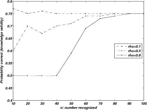
| Figure 4: Probability correct, given both items are recognized, for
LINDA as a function of n and ρ. This is equivalent to
Goldstein and Gigerenzer’s (2002) concept of knowledge
validity. |
As expected, the RH model’s performance when just one of the two items
is recognized improves with ρ . This is also true for the high
quality knowledge version of LINDA (pA = pB = pC =1) and the
same effect is present but in a weaker form for the low quality
knowledge version of LINDA (pA = pB = pC = 0.7). Crucially,
the performance of both models varies with n. These results show
formally that observed recognition validity, as assessed from actual
performance, can vary according to other aspects of an individual’s
knowledge. This effect is particularly marked for large ρ . Next,
consider knowledge validity. Similarly to recognition validity, the
conditional probability of a correct inference given that both items
are recognized can be derived and is expressed in our notation as
follows:
|
| | α110 p110 + α101 p101 + α011 p011 |
|
| p110 +
p101 + p011 |
|
(3) |
Figure 4 shows probabilities of correct inference, conditional on
recognizing both items of a stimulus pair (knowledge validity), for
LINDA, varying recognition-magnitude correlations. This is the high
quality knowledge with pA = pB = pC =1, a lower quality
knowledge version with pA = pB = pC =0.7 produces lower levels
of performance overall but almost identical patterns in response to
the same variations in n and ρ . Knowledge validity for
situations in which the RH is the object of attention is often set at
an arbitrary value (e.g., Goldstein & Gigerenzer, 2002; Schooler &
Hertwig, 2005) but we would expect it to vary as a function of n and
ρ for many knowledge-based heuristics, as it does for LINDA,
although the specifics will depend upon the exact nature of the
inference rule.
In conclusion, finding LiMEs is dependent not only upon identifying the
decision rule and circumstances under which they are expected but also
upon accurately estimating — or manipulating — n in order to
obtain the recognition- and knowledge-validity parameters required.
Given this, it is perhaps less surprising than it initially appeared
that such effects, which would appear to be a mathematical necessity,
may sometimes be elusive when investigated empirically.
3 General discussion
The aim of the current paper was not to present unequivocal support
for LINDA as in some way a better, more accurate, or more comprehensive
model of decision-making than the RH, or to refute the RH as a model
(indeed, it has proven far more productive than its underlying
simplicity might lead one to believe). We have instead attempted to
meet the rather more modest aim of giving an existence-proof that,
generally, disentangling recognition from other forms of information is
more difficult than it may first appear. In this context, LINDA is best
viewed as an analytical tool to enable us to make these arguments in a
mathematically rigorous way. The counter-intuitive nature of LiMEs was
previously viewed as providing a strong test of recognition-driven
inference given that LiMEs are predicted by the RH. This position is
weakened by the demonstration that LiMEs can easily be produced using a
set of assumptions in which recognition-only inference plays no part.
Criticisms of LiMEs as a means of promoting recognition-driven inference
could perhaps be interpreted as an argument against the proposal that
inference might sometimes be recognition-driven. It should be
emphasized that this was not the intent. Rather, we wished to provide a
demonstration that findings which initially seem favorable to such a
position may not necessarily be as conclusive as they first appear. The
absence, as well as the presence, of LiMEs is also less informative
than some have assumed (e.g., Boyd, 2001; Dougherty et al., 2008; Pohl,
2006), and for similar reasons. The recognition validities for both
recognition-consistent and recognition-driven inferences are similarly
dependent upon variations in n, which is not ordinarily under
experimental control. For at least one form of knowledge-based
inference (that of LINDA) knowledge validity itself is also a function
of n. It is possible therefore that both published
demonstrations of LiMEs and published failures to obtain such an effect
employed different de facto recognition and knowledge
validities than those assumed a priori. A positive
contribution therefore is to suggest that future studies along these
lines will need to take such factors into account.
Finally, LINDA can be applied either in tandem or in opposition to the
RH. For example, the rule “Apply knowledge (e.g., LINDA) if both
items are recognized and apply the RH if only one item is recognized”
is standard procedure for many heuristics (e.g., Gigerenzer &
Goldstein, 1996, examined six different procedures that made use of
the recognition principle when knowledge failed and only one item was
recognized). However, “Apply LINDA whenever possible but if LINDA
does not provide usable information for this item, apply the RH” is
also a valid strategy and one which might prove superior if LINDA is
particularly reliable. This latter statement reduces to the assertion
that a minimal level of confirmation or refutation will be sought when
only one item is recognized and that “mere” recognition will be
employed only if and when this minimal test fails to produce usable
knowledge. This assertion is consistent with recent data by Hilbig and Pohl
(2008).
In the current formulation, LINDA always has access to median knowledge
for the recognized items (though this information may not always be
correct). Other LINDA-like models could be developed where some
recognized items may not have median knowledge associated with them,
although we do not go into detail about such items here. The key
difference between LINDA and the recognition heuristic is that
sometimes LINDA recognizes items which it believes are below median.
This enables it to guess correctly, in situations where only one item
is recognized, that the recognized item is the smaller of the pair. In
contrast, provided the magnitude-recognition correlation is positive,
the RH always guesses that the recognized item is larger (the converse
also applies: where the magnitude-recognition correlation is negative,
the RH will always guess that the recognized item is smaller whereas
LINDA will sometimes know better). In circumstances where LINDA
believes all the items it recognizes are above median, LINDA and the RH
make identical predictions. There is nothing magical about using median
knowledge in our modeling, it is simply a tractable way of
characterizing limited information. Any model that has the property
that it knows that some of the items it recognizes are small, but in
general has very limited information, is likely to behave in a
LINDA-like manner.
References
Borges, B., Goldstein, D. G., Ortmann, A., & Gigerenzer, G. (1999). Can
ignorance beat the stock market? In: G. Gigerenzer, P. M. Todd, & the
ABC Research Group (Eds.). Simple heuristics that make us
smart. Oxford: Oxford University Press.
Boyd, M. (2001). On ignorance, intuition and investing: A bear market
test of the recognition heuristic. Journal of Psychology and
Financial Markets, 2, 150–156.
Dougherty, M. R., Franco-Watkins, A. M., & Thomas, R. (2008).
Psychological plausibility of the theory of probabilistic mental models
and the fast and frugal heuristics. Psychological Review, 115,
199–213.
Frosch, C., Beaman, C. P., & McCloy, R. (2007). A little learning is a
dangerous thing: An experimental demonstration of ignorance-driven
inference. Quarterly Journal of Experimental Psychology,
60, 1329–1336.
Gigerenzer, G. (2007). Gut feelings: The intelligence of the
unconscious. New York: Viking Press.
Gigerenzer, G., & Brighton, H. (2009). Homo heuristicus: Why biased
minds make better inferences. Topics in Cognitive Science, 1,
107–144.
Gigerenzer, G., & Goldstein, D. G. (1996). Reasoning the fast and
frugal way: Models of bounded rationality. Psychological
Review, 103, 650–669.
Goldstein, D. G., & Gigerenzer, G. (2002). Models of ecological
rationality: The recognition heuristic. Psychological Review,
109, 75–90.
Hilbig, B. E., Erdfelder, E., & Pohl, R. F. (2010). One reason
decision-making unveiled: A measurement model of the recognition
heuristic. Journal of Experimental Psychology: Learning, Memory
& Cognition, 36, 123–134.
Hilbig, B. E., & Pohl, R. F. (2008). Recognizing users of the
recognition heuristic. Experimental Psychology, 55, 394–401.
Hilbig, B. E., Pohl, R. F., & Bröder, A. (2009). Criterion knowledge:
A moderator of using the recognition heuristic? Journal of
Behavioral Decision Making, 22, 510–522.
McCloy, R., Beaman, C. P., Frosch, C., & Goddard, K. (2010). Fast and
frugal framing effects? Journal of Experimental Psychology:
Learning, Memory & Cognition, 36, 1042–1052.
McCloy, R., Beaman, C. P., & Smith, P. T. (2008). The relative success
of recognition-based inference in multi-choice decisions.
Cognitive Science, 32, 1037–1048
Newell, B. R., & Fernandez, D. (2006). On the binary quality of
recognition and the inconsequentiality of further knowledge: two
critical tests of the recognition heuristic. Journal of
Experimental Psychology: Learning, Memory & Cognition, 19, 333–346.
Newell, B. R., & Shanks, D. R. (2004). On the role of recognition in
decision-making. Journal of Experimental Psychology: Learning,
Memory & Cognition, 30, 923–935.
Pachur, T., & Biele, G. (2007). Forecasting from ignorance: The use and
usefulness of recognition in lay predictions of sports events.
Acta Psychologica, 125, 99–116.
Pachur, T., Bröder, A., & Marewski, J. (2008). The recognition
heuristic in memory-based inference: Is recognition a non-compensatory
cue? Journal of Behavioral Decision-Making, 21, 183–210.
Pachur, T. & Hertwig, R. (2006). On the psychology of the recognition
heuristic: Retrieval primacy as a key determinant of its use.
Journal of Experimental Psychology: Learning, Memory &
Cognition, 32, 983–1002.
Pachur, T., Mata, R., & Schooler, L. J. (2009). Cognitive aging and the
adaptive use of recognition in decision making. Psychology &
Aging, 24, 901–915.
Pohl, R. F. (2006). Empirical tests of the recognition heuristic.
Journal of Behavioral Decision-Making, 19, 251–271.
Reimer, T., & Katsikopoulos, K. (2004). The use of recognition in group
decision-making. Cognitive Science, 28, 1009–1029.
Richter, T., & Späth, P. (2006). Recognition is used as one cue among
others in judgment and decision making. Journal of Experimental
Psychology: Learning, Memory & Cognition, 32, 150–162.
Schooler, L. J., & Hertwig, R. (2005). How forgetting aids heuristic
inference. Psychological Review, 112, 610–628.
Snook, B., & Cullen, R. M. (2006). Recognizing national hockey league
greatness with an ignorant heuristic. Canadian Journal of
Experimental Psychology, 60, 33–43
Volz, K. G. , Scholler, L. J., Schubotz, R. M., Raab, M., Gigerenzer,
G., & von Cramon, D. Y. (2006). Why you think Milan is larger than
Modena: Neural correlates of the recognition heuristic. Journal
of Cognitive Neuroscience, 18, 1924–1936.
Appendix
1. Derivation of the values of pijk in Equation (1): A total
sample of N = 100 items is assumed, of which n are recognized. n
is systematically varied between 0–100 in all the studies reported
here.
u, v and w are the numbers of items recognized from
each of the subsets A (comprising items only from the top
quartile), B (second quartile) and C (below median).
These can be used to calculate n.
The probabilities associated with recognizing 0, 1 or 2 items from
u, v and w on any given trial
(pijk) can then be calculated as follows:
Probabilities associated with recognizing none of the items from
u, v or w:
|
| | p000 | | | | | | | | | | |
| | | = | | (N − u − v − w) (N − u − v − w − 1) |
|
| N(N − 1) |
|
| | | | | | | | | |
|
Probabilities associated with the recognition of only one item:
| p100 = | | · | | = | | 2u(N − u
− v − w) |
|
| N(N − 1) |
| |
This is the probability that only one of the two items is recognized and
it is in the top quartile (a member of u).
Probabilities that the item recognized is from the second quartile, or
is below the median, and that the other item is not recognized can be
calculated by substituting v or w, respectively, for
u in the first term, giving:
Probabilities associated with the recognition of both items:
(for u and v, so one item is in the top quartile and
one item is in the second quartile)
(as above, substituting v and w where appropriate)
(where both items are in the top quartile, both are members of
u)
(as above, substituting v and w where appropriate).
2. Parameters for the Recognition Heuristic model. These
represent the calculated probabilities of success associated with
recognizing 0, 1 or 2 items where the appropriate probabilities of
recognizing 0, 1 or 2 items are given by the equations calculated in
section 1 of this appendix. Overall performance of each of the
strategies (the RH and LINDA) is then given by equation (1)
Recognize none:
α000 = 0.5 (Chance)
Recognize one item (which happens to be in the top quartile, i.e., a
member of u):
|
| | α100 | | = 0.5 · | | +
| | 0.75N − v − w |
|
| N − u − v − w |
| |
| | | | | | | | | |
| | | = | | 0.875N − 0.5u − v − w |
|
| N − u − v − w |
|
| | | | | | | | | |
|
For recognition of members of v and w, the chances of
success are similarly:
|
| | α010 | | | | | | | | | | |
| | | = | | 0.625N − u − v − w |
|
| N − u − v − w |
|
| | | | | | | | | |
|
The recognized item is in the second quartile.
| α001 = 0 + 0.5 | | =
| | 0.25N − 0.5w |
|
| N − u − v − w |
| |
The recognized item is below median.
For all these cases which involve recognition of both items
α110 = α101 = α011 = α200 = α020 = α002
It is assumed knowledge can be used with a certain probability of
success. This probability is chosen to make the LINDA and RH models
“equivalent” in our examples, in the sense that they both produce
the same probability of success when all items are recognized.
3. Parameters for the LINDA model. These represent the calculated
probabilities of success associated with recognizing 0, 1 or 2 items
where the appropriate probabilities of recognizing 0, 1 or 2 items are
given by the equations calculated in section 1 of this appendix. The
means of deriving these equations is basic probability theory similar
to that used to obtain the corresponding values for the Recognition
Heuristic, although the equations themselves are necessarily more
complex and therefore explained in a little more detail. Overall
performance of the LINDA model is given by Equation 1.
Recognize none:
α000 = 0.5 (Chance).
Recognize one item:
|
pA · | | 0.75 N − v − w |
|
| N − u − v − w |
| + |
|
= | | 0.5 · (0.25N − u) + pA · (0.75 N − v − w) |
|
| N − u − v − w |
|
The participant recognizes one item, which is from the top quartile.
With probability pA they
believe it to be above median and choose it.
The first term is then the probability that the non-recognized item is
also in the top quartile, times the probability of success (chance).
The second term is the probability that the non-recognized item is in
the second quartile or lower, times the probability of success.
With probability 1 − pA the
participant believes the recognized item is below median, and so does
not choose it.
The third term is the probability that the non-recognized item is in the
top quartile, with chance probability of being correct.
The fourth term is the probability that the non-recognized item is in
the second quartile or lower, with no chance of being correct.
The probability of choosing correctly if one item from u is
recognized is the sum of these terms and the second line of the
equation rewrites the calculation for overall probability of success
into a more succinct form. The equations for choosing correctly when a
single item from v or w is recognized take similar
form:
|
= | | 0.375N − u − 0.5v + pB · ( 0.25N + u −w) |
|
| N − u − v − w |
|
The recognized item is in the second quartile (from v). With
probability pB they believe it is above median.
|
α001 = 0 + (1−pC) · 0.5 · | | + |
|
pC · | | 0.5N − u −v |
|
| N − u − v − w |
| + |
|
= | | 0.25 N − 0.5 w + pC · (0.5 N − u − v) |
|
| N − u − v − w |
|
The recognized item is below median (from w). With probability 1−
pC the participant believes the item is above median.
Two items are recognized.
With reference to u, v, w, the possible combinations in which
this might occur are: 110, 101, 011, 200, 020, 002.
If two items are recognized and one item is in the first quartile
(from u) and the second item is in the second quartile (from
v). With probability pA the participant believes the first item
is above median and with probability pB they believe the second
item is above median. This then gives the following derivation:
|
| | α110 | = 0.5 pA pB + pA (1 − pB) + | | | | | | | | | |
| | 0 + 0.5 (1 − pA) (1 −pB) | | | | | | | | | |
| | = 0.5 + 0.5 pA − 0.5 pB
| | | | | | | | | |
|
Calculations for the other ways in which two items might be recognized
(e.g., one item from the top quartile and one from below the median)
can similarly be combined with the parameters pA, pB and pC
as follows:
α101 = 0.5 +0.5 pA − 0.5(1−pC) = 0.5 pA + 0.5pC
(As above, substituting 1−pC for pB)
α011 = 0.5pB + 0.5 pC
(As above, substituting pB for pA)
α200 = α020 = α002 = 0.5
Both items are from the same subset, and so cannot be distinguished,
performance is chance.
This document was translated from LATEX by
HEVEA.