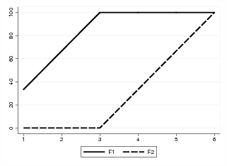
| Figure 1: Cumulative distribution functions of religious frequency for two samples. |

Judgment and Decision Making, vol. 5, no. 2, April 2010, pp. 176-181
Incentives in religious performance: a stochastic dominance approachTeresa García-Muñoz* |
Using a stochastic dominance approach in an international dataset of about 10,000 Catholic subjects, we show that incentives (based on absolute belief) play a crucial role in religious practice (church attendance and prayer). Furthermore, we find that when both positive (heaven) and negative (hell) incentives are available, the former have a much stronger effect than the latter. The results are confirmed using Kolmogorov-Smirnov tests.
Keywords: incentives, rewards, punishment, economics of religion.
Many studies have examined the role of incentives and their effect on the behavior of individuals (Tversky & Kahneman, 1991; Slonim & Roth, 1998; Andreoni et al., 2003; Nikiforakis, 2008; among others). In this study, the interest falls on the effect of incentives on religious behavior in the sense that they increase (decrease) individual religious performance.
Religious practice can be encouraged by two types of incentives: earthly ones and afterlife ones.
This paper addresses the second group. Previous studies have analyzed the effects of “afterlife incentives” on religious behavior. Azzi and Ehrenberg (1975) were the first to propose and test a theoretical model of afterlife religious capital.1 They analyzed the determinants of participation in religious activities using a utility-maximizing model. Among other results, they found afterlife beliefs to be a major determinant of church attendance. Using several surveys carried out in the United States, they provided empirical support for their theory.
Blomberg et al. (2006) developed a model where financial religious contributions are motivated by both current consumption and afterlife considerations. They show that afterlife considerations play an important role in explaining financial religious contributions.
Pyne (2010) studied the relationship between religiosity and the fear of death. He found that individuals who place a higher probability on the existence of an afterlife invest more in religious capital.
Recently, Brañas-Garza et al. (2010) estimated the role of afterlife beliefs in the production of religious commodities, concretely, church attendance and prayer. Using ordered logit regressions, they found that afterlife beliefs are crucial determinants but, more importantly, that beliefs in heaven are much more relevant than beliefs in hell: positive incentives are stronger than negative ones. However, this regression approach does not allow us to study the joint effect of positive and negative incentives. When the logit model contains interactions (among variables) two problems appear: i) the computation of partial effects becomes problematic; ii) the interpretation of these estimate effects is not straightforward. As showed in Norton et al. (2004) the estimated coefficients of the interaction terms do not reflect the interaction effect; moreover their statistical significance cannot be tested through a simple t-test. Even more problematic is the interpretation given that the estimated interaction effect is also conditional on the current value of the other independent variables. Hence, we cannot properly study the meaning of different interactions in a logit regression model.
This paper presents a different statistical tool — the stochastic dominance approach (Levy, 1998) — that allows the use and the straightforward interpretation of the joint effect of positive and negative incentives. Our analyses confirm the main results showed in Brañas-Garza et al. (2010) and revises the interactive effects among positive and negative incentives. In an easy and graphical way we show that afterlife incentives play a crucial role in religious performance, comparing not only and positive or negative incentives but combination of both are compared.
The study was carried out on Catholic people. In the Catholic religion, church attendance and prayer are strategies that lead to heaven and prevent hell. Church attendance and prayer are two dimensions of religiosity that reflect public religious activities versus private/intimate prayer activities. While church attendance also has non-religious motives such as networking and the building of social ties, private prayer activity has more pure religious motives.
Using a stochastic dominance approach, we ask whether absolute beliefs in eternal bliss (heaven) and in eternal damnation (hell) increase individual’s religious investment as reflected in church attendance and prayer, and whether absolute belief in eternal damnation (hell) is a more or less powerful incentive than eternal bliss (heaven) for intensified religious effort.
The data were drawn from the module on National Identity of the 1998 International Social Survey Program (ISSP): Religion II. The survey contains questions about attitude and beliefs, specifically:
The last three questions have the same four options: (1) yes, definitely; (2) yes, probably; (3) no, probably not; and (4) no, definitely not.
The promise of an afterlife serves as an incentive for believers to engage in religious behavior. Those who definitely believe in heaven are confident that they will be highly rewarded, thus belief in heaven can be considered a positive incentive (with p=1). On the opposite side, those who definitely believe in hell are confident that they will be highly punished after death. Therefore, belief in hell can be considered a negative incentive (with p=1).
After excluding respondents who did not answer some of the questions, the final dataset was comprised of about 10,840 Catholic subjects. Table 1 shows their distribution of beliefs:
Table 1: Distributions of beliefs for Catholics (%)
Afterlife after death Heaven Hell Yes, definitely 35.77 34.73 25.72 Yes, probably 33.43 31.78 25.84 No, probably not 13.77 15.71 21.88 No, definitely not 17.02 17.78 26.56
Table 1 reveals that afterlife incentives are important (the largest category is shown in bold). As can be seen, individuals are concerned with what happens after death, although the people that believe in a reward (heaven) are much more numerous than those who believe in a punishment (hell). On average, subjects are optimistic regarding afterlife outcomes.
Concerning beliefs about heaven and hell, Table 2 shows the contingency table of the responses by 10,840 subjects.
Table 2: Contingency table of responses of 10,840 subjects.
Do you believe in hell? Yes, definitely Yes, probably No, probably not No, definitely not Do you believe in heaven? Yes, definitely 2,726 423 239 377 3,765 Yes, probably 46 2,347 657 395 3,445 No, probably not 5 25 1,465 208 1,703 No, definitely not 11 6 11 1,899 1,927 2,788 2,801 2,372 2,879 10,840
Since we focus only on people who definitely believe or definitely do not believe (that is, the subjects appearing in bold in Table 2), the sample is reduced to 5,013 subjects.
Hence, we define a 2x2 factors design according to the type of incentives affecting subjects. As shown in Table 2 (in bold), we have:
Using a stochastic dominance approach and the Kolmogorov-Smirnov test, we compare individual religious performance (church attendance and prayer) according to the type of incentive affecting each person. Basically, we compare the respondents with both types of incentives versus respondents with only positive incentives versus respondents with no incentives.
Stochastic dominance is an abbreviated term for first-order stochastic dominance, which refers to a set of relations that may hold between a pair of distributions (Levy, 1998). Stochastic dominance is usually applied to the analysis of income distribution and income inequality (for example, Davidson, 2006, and Davidson & Duclos, 2000). The concept can, however, be applied in many other domains. Concretely, we can study the effectiveness of several incentives on church attendance and prayer using the stochastic dominance relation between the distributions of these two variables generated by these incentives.
In order to determine whether a relation of stochastic dominance holds between two distributions, the distributions are first characterized by their Cumulative Distribution Functions (CDF). For instance, in the previous section we saw that the question about church attendance has 6 response levels ranging from “never (1)” to “at least once a week (6)”. For a given sample, the value of the CDF at level a is the proportion of subjects in the sample that do not go to church more than a.
Suppose we find the following “radical” situation. We have two different samples of subjects. The people in the first sample are not so religious (in terms of church attendance), while in the second sample, subjects attend church very frequently. The relative frequencies and CDFs for each level of church attendance for both samples are presented in Table 3.
Table 3: Relative frequencies and CDFs for each level of church attendance for both samples.
Sample 1 Sample 2 % CDF (F1) % CDF (F2) Never (1) 33.33 33.33 0 0 Once a year (2) 33.33 66.67 0 0 2 or 3 times a year (3) 33.33 100 0 0 Once a month (4) 0 100 33.33 33.33 2 or 3 times a month (5) 0 100 33.33 66.67 At least once a week (6) 0 100 33.33 100
Clearly, the second sample contains subjects who engage in religious practices with greater frequency. Figure 1 shows the cumulative distribution functions of these two samples.
Figure 1: Cumulative distribution functions of religious frequency for two samples. 
Let us now introduce the concept of stochastic dominance.
Definition 1
Suppose that we consider two distributions A and B, characterized respectively by the cumulative distribution functions FA and FB. Then distribution B dominates distribution A stochastically (at the first order) if, for any argument a, FB(a)≤ FA(a).
In our example, inequality is F2(a)≤ F1(a), for all a, that is, the distribution of church attendance in the second sample stochastically dominates (is always below) the distribution in sample 1. This means that the proportion of subjects in each level in F2 is always less than or equal to the proportion of subjects in each level in F1.
In other words, Sample 2 is formed by more religious people (in terms of church attendance) than Sample 1. For this reason we say that the second sample “dominates” the first one since Sample 2 has more subjects in the upper categories of the ordinal variable we are studying (church attendance)2.
With this type of data, where the distribution functions do not cross in any point, the criterion of first order dominance allow to compare the behavior of several sub-samples in an easy and graphical way. In addition, this method does not demand any hypothesis about the distribution shape, and it uses all the points of the distribution.
In the next section we use this approach to explore the effect of incentives on religious performance.
In Section 2 we selected 5,002 Catholic subjects who definitely believe or definitely do not believe in heaven and hell. The subjects have been divided into three samples according to what types of incentives (beliefs) affect them: people affected by both incentives (heaven and hell), people affected by the positive incentive only (heaven) and people with no incentives. In Tables 4 and 5, the CDFs of church attendance and prayer are given for the three samples:
Table 4: CDFs of attendance.
Positive and negative incentives Positive incentives only No incentives Never (1) Once a year (2) 2 or 3 times a year (3) Once a month (4) 2 or 3 times a month (5) At least once a week (6)
Table 5: CDFs of prayer.
Pos. and neg. incentives Positive incentives only No incentives Never (1) Once a year (2) Twice a year (3) A few times a year (4) About once a month (5) Two or three times a month (6) Almost every week (7) Every week (8) Several times a week (9) Once a day (10) Several times a day (11)
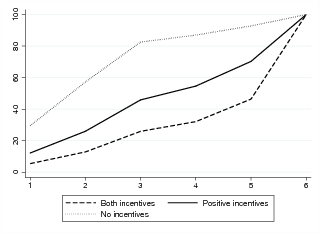
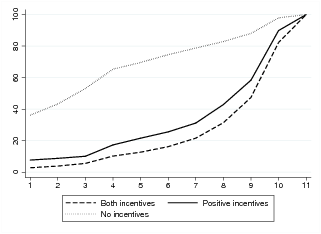
Figures 2 and 3 show the cumulative distribution functions. In both figures, the “both incentives” distribution was found to stochastically dominate the “no incentives” and “positive incentives” distributions. Moreover, the “positive incentives” distribution stochastically dominates the “no incentives” distribution. At all attendance and prayer levels, the CDF values of “both incentives” are smaller than the CDF values of the other two samples. As we explained in Section 3, this means that there is a higher proportion of practicing subjects (church attendance and prayer) among people who are affected by negative and positive incentives than in the other groups.
Figure 2: CDFs for attendance 
Figure 3: CDFs for prayer.

The differences between distributions can be statistically corroborated using the Kolmogorov-Smirnov test.3 In Table 6 we present the statistics and significance of this test to compare the distributions of church attendance and prayer among the three samples:
In sum, we find that:
Furthermore, the positive incentives effect is large, whereas the negative incentives effect is smaller. We obtain this result by comparing the net effects of “both incentives” versus the net effect of “positive incentives only”. When we remove the “negative incentives” effect, that is, when we jump from the “both incentives” sample to the “positive incentives” sample, attendance and prayer distributions are closer than when we remove the “both incentives” effect, that is, when we jump from the “positive incentives” sample to the “no incentives” sample. This can be viewed graphically in Figures 2 and 3 and by numerically calculating the mean differences between the CDF values.
For attendance distribution, the Mean Differences (MD) are:4
MDNo−Positive=
1/5∑i=15 ( CDFNo(i)−CDFPositive(i)) = 28.08
MDPositive−Both=
1/5 ∑i=15 ( CDFPositive(i)−CDFBoth(i)) = 17.25
We observe that the distance between the “positive incentives” distribution and the “no incentives” distribution is larger than the distance between the “positive incentives” and “both incentives” distributions.
For prayer distribution, the mean differences are:
MDNo−Positive =
1/10 ∑i=110 [ CDFNo(i)−CDFPositive(i)] = 37.63
MDPositive−Both =
1/10 ∑i=110 [ CDFPositive(i)−CDFBoth(i)] = 7.93
The “positive incentives” effect is stronger for prayer than for
attendance distribution. When we only remove the “negative
incentives” effect (jumping from the “both incentives” sample to
the “positive incentives” sample), the behavior of the prayer
distribution is similar in both samples (the MD between both CDFs is
7.93).
Table 6: Kolmogorov-Smirnov tests (p-values in parentheses). Positive incentives only.
0.2392 (0.000) 0.1152 (0.000) 0.3668 (0.000) 0.4898 (0.000)
Using a stochastic dominance approach and a dataset of 10,840 Catholic subjects, we have illustrated that incentives have a major effect on religious behavior and that positive incentives have a much stronger effect than negative ones when both types of incentives are available. This result is similar to the one proposed in the cooperation experiments described in Andreoni et al. (2003) and contributes to the robustness of the estimated effects of positive/negative religious incentives in Brañas-Garza et al. (2010).
Therefore we may conclude that:
In sum, our study supports the pronounced effectiveness of positive rewards, but finds no large effects for punishment. Hence we may conclude that the Catholic Church could be much more successful in their performance (aggregate behavior) if it were to promote heavensward activities rather than the fear of God.
Andreoni, J., Harbaugh, W., & Vesterlund, L. (2003). The carrot or the stick: rewards, punishments, and cooperation. American Economic Review, 93, 893–902.
Azzi, C. & Ehrenberg, R. (1975). Household allocation of time and church attendance. The Journal of Political Economy, 83, 27–56.
Brañas-Garza, P., García-Muñoz, T. & Neuman, S. (2010, forthcoming). The big carrot: high-stake incentives revisited. Journal of Behavioural Decision Making.
Blomberg, S., DeLeire, T. & Hess, G. D. (2006). The afterlife-cycle theory of religious contributions. CESinfo Working Paper no. 1854.
Davidson, R. (2006). Stochastic dominance. The new Palgrave dictionary of Economics. Second Edition. Eds. Steven N. Durlauf and Lawrence E. Blume. Palgrave Macmillan.
Davidson, R., & Duclos, J. Y. (2000). Statistical inference for stochastic dominance and for the measurement of poverty and inequality. Econometrica, 68, 1435–1464.
Levy, H. (1998). Stochastic dominance. Kluwer Academic Publishers, Norwell, MA.
Nikiforakis, N. (2008). Punishment and counter-punishment in public good games: can we really govern ourselves? Journal of Public Economics, 92, 91–112.
Norton, E. C., Wang, H. & Ai, C. (2004). Computing interaction effects and standard errors in logit and probit models. The Stata Journal, 4 , 154–167.
Pascal, B. (1670). Pensées de M. Pascal sur la religion, et sur quelques autres sujets.
Pyne, D. (2010). A model of religion and death. Journal of Socio-Economics, 39, 46–54.
Slonim, R., & Roth, A. E. (1998). Learning in high-stakes ultimatum games: an experiment in the Slovak Republic. Econometrica, 66, 569–596.
Tversky, A., & Kahneman, D. (1991). Loss aversion in riskless choice: a reference dependent model. Quarterly Journal of Economics, 106, 1039–1061.
This document was translated from LATEX by HEVEA.