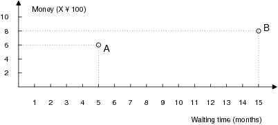
| Figure 1: The waiting time salient version of the scholarship problem. |
Judgment and Decision Making, vol. 5, no. 3, June 2010, pp. 151-158
Attribute salience in graphical representations affects evaluationYan Sun* and Shu Li |
By manipulating the scale in graphs, this study demonstrated a new evaluation bias caused by attribute salience in graphical representations. That is, (de)compressing the graph axis scale changed the relative distance with respect to the options of a given attribute and thus changed the salience of the information in graphical representations. Experiment 1 showed that the differences in the graphical representations had a significant impact on the evaluation. Experiment 2 repeated the scale manipulation effect in a different scenario and extended it to a multi-options context. Experiment 3 disentangled the effect of scale distance manipulation from the other variables (e.g., scale resolution and assignment of attributes to axes) and further supported the finding of Experiment 1. These results indicated that attribute salience in graphical representations clearly affects evaluations and that graphs can be manipulated to cause very different impressions of the same data. This finding is not consistent with the axioms of normative economic theory. Experiment 3 also tested the attribute importance hypothesis, but the evidence indicated that the participants did not regard the longer axis as the more important attribute. Finally, we related our findings to the impact of visual processing on decision making and discussed them from the perspective of two-system cognitive theory.
Keywords: scale manipulation, focus bias, salience, graphical
representation, judgment and decision making.
People often focus on a single, salient aspect of a problem and overlook the rest when making a decision. Such a limited focus can cause a bias in the decision making process and leads to results that violate the axioms of normative economic theory. Interestingly, incidental information (e.g., the way that preferences are elicited and the wording of the options) could in some cases determine which information is perceived as salient, and thus what people would focus on in decision making situations.
Evidence has indicated that the means of preference elicitation (e.g., choose vs. reject) is likely to shift the focus of decision makers. In a hypothetical sole-custody case, Shafir (1993) found that people who had the option to choose tended to focus on the parents’ positive attributes; whereas people who were asked to reject tended to focus on the parents’ negative attributes. As a result, a preference-reversal occurs when the same enriched option was the majority choice for both choosing and rejecting.
In line with this focusing view, Jones, Frisch, Yurak, and Kim (1998) reported an interesting framing effect caused by the description of the options. When the decision was described as choice (e.g., Should I move to New York or stay in Chicago?), people paid equal attention to each of the options. However, when the same decision was described as opportunity (e.g., Should I move to New York?), people focused their attention on the single option that was explicitly mentioned. Thus preference was changed when the opportunity description made the single option more salient.
Figure 1: The waiting time salient version of the scholarship problem. 
Figure 2: The money amount salient version of the scholarship problem. 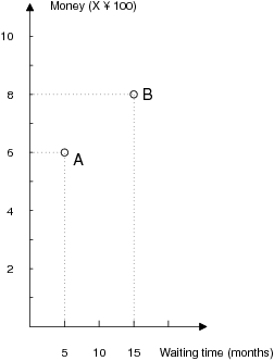
Levin (1987) and Levin and Gaeth (1988) evaluated the associative effects of various ways of framing consumer information and found that the consumers’ evaluations were more favorable toward beef labeled “75% lean” than to that labeled “25% fat”, because the information about the lean percentage was salient in the former but not in the latter. Kahneman and Tversky (1984) found that there was a pseudo-certainty effect in a two-stage risky choice, showing that individuals tended to neglect an earlier contingency and only focus on the second (contingent) decision. Recently, Li, Su and Sun (2010) reported a similar pseudo-immediacy effect in a two-stage intertemporal choice.
Interestingly, people also tend to make biased spatial judgments as a result of focusing only on the most salient aspects of spatial stimuli, ignoring other dimensions. For example, Piaget (1968) found that children appeared to use only the height of a container when making volume judgments and ignored the diameter of the cylinder. Raghubir and Krishna (1999) even found similar results with adults. Verge and Bogartz (1978) asked children to adjust a square to match the area of a rectangle and found that the majority of children tended to equate the side of the square with either the width or the height of the rectangle and neglect the other relevant dimension. Similarly, Raghubir and Krishna (1996) found that people often use the direct distance between the endpoints of a nonstraight path as a proxy for distance judgment, with little regard for the path configuration. In a recent study, this direct distance bias was even able to be found in a real stock market situation, in which the information was presented using graphs. The stocks with the higher run lengths were often perceived as riskier (Raghubir & Das, 2010).
Since people often focus on the most salient aspects in spatial judgments and tend to be biased by the focus of attention in choice, as reviewed above, we conjectured that the focusing bias would also appear in decision making problems presented with graphs, if we manipulated the graphical representations of the options. In order to appreciate the significance of this manipulation, see the Scholarship problem in Figures 1 and 2, in which the same information is provided in each figure, but the salience of the information in the spatial (graphical) representation differs as a function of the scale employed in each of the graphs. That is, the waiting time attribute appears to be relatively salient in Figure 1; whereas the money amount attribute appears to be relatively salient in Figure 2.
Imagine that, you applied for a scholarship. [Two types of scholarships (A, B) were presented with graphs involving two attributes (money amounts and waiting time).] Obviously, you would be glad if you could get a scholarship with less waiting time but more money. On the basis of the following data, please indicate your preference strength on a 9-point scale ranging from 1 (not at all) to 9 (extremely) for each type of scholarship.
We hypothesized that the evaluation of the two types would be affected by the scale employed in the graphs, since people tend to focus on the salient attribute. Specifically, the preference strength for type A would be higher in participants who saw Figure 1 than in those who saw Figure 2, but the reverse would be true for type B. The following Experiment 1 carried out this test of the scale effect.
The initial participant pool consisted of 195 undergraduate student volunteers who were recruited by poster, and all of whom provided oral consent. All participants were given a small gift for their participation, but two incomplete questionnaires were excluded from the analysis.
The Scholarship problem, along with several other unrelated problems, was presented in questionnaire form in two versions (i.e., a waiting time salient version and a money amount salient version). The two versions were identical, except that a different scale was employed in the figures. That is, Figure 1 was used in the waiting time salient version; whereas Figure 2 was used in the money amount salient version. The participants, randomly assigned to one of the two versions, were asked to rate their preference strength on a 9-point scale ranging from 1 (not at all) to 9 (extremely) for each type of scholarship. In the end, 99 participants responded to the waiting time salient version; whereas the remaining 94 participants responded to the money amount salient version. Thus, this is a 2 (scholarship type: type A vs. type B) × 2 (graph version: the waiting time salient version vs. the money amount salient version) mixed experimental design, with the graph version as the between-subjects factor and the scholarship type as the within-subjects factor. The dependent variable was the preference strength for a scholarship.
In order to check the effect of scale manipulation on spatial perception, we removed the numbers and labels from Figures 1 and 2. We presented an additional 19 participants with these blank figures and asked them to rate “the difference in the distance between A and B along the X-axis/Y-axis” on a 9-point scale ranging from 1 (very small) to 9 (very large) for each figure. The results showed that the rated score was higher for the X-axis (M = 8.211) than for the Y-axis (M = 3.110) for Figure 1 (t(18) = 12.011, p < .001) whereas the rated score difference was not significant between the X-axis (M = 4.368) and the Y-axis (M = 4.684) for Figure 2 (t(18) = -1.372, p > .05). This result thus indicated that our scale manipulation was effective with respect to spatial perception.
A 2×2 ANOVA on preference strength revealed that the main effect was significant for scholarship type, F (1, 191) = 6.709, p < .05. More relevant to this study is that the ANOVA also showed a significant interaction between scholarship type and graph version, F (1, 191) = 5.048, p < .05, indicating that the effect of scholarship type on preference strength was influenced by the graph version. In fact, type A (M = 6.889, N=99) was preferred over type B (M = 5.990, N=99) in the waiting time salient version, t (98) = 3.330, p < .01. However, the relative preference of type A (M = 6.266, N=94) over type B (M = 6.202, N=94) was non-significant in the money amount salient version, t (93) = 0.251, p > .05.
As we predicted, these results indicated a stronger preference of type A over type B in Figure 1, compared to Figure 2. Contrary to the principle of invariance, the result of our Experiment 1 indicated that simply compressing the scale in a graph can yield systematic fluctuations in the evaluation, even if the same information is presented.
Experiment 1 confirmed that the participants’ evaluations would be affected by the scale employed in graphs. However, perhaps the scale manipulation effect can be obtained only in situations in which just two options are made available. Indeed, only two options were presented to participants in Experiment 1. Thus, whether the scale manipulation effect can be extended to multi-options conditions needs clarification. Evidence has demonstrated that varying the number of options can shift the preference in decision making (Jones, Frisch, Yurak & Kim, 1998; Tversy, Slovic, & Kahneman, 1990). The purpose of Experiment 2 was to test the generalization of the scale manipulation effect in a multi-options context.
Figure 3: The technical knowledge salient version of the employee problem. 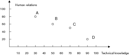
Figure 4: The human relations salient version of the employee problem. 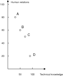
The initial participant pool consisted of 176 undergraduate student volunteers who were recruited by poster, and all of whom provided oral consent. All participants were given a small gift for their participation, but two incomplete questionnaires were excluded from the analysis.
An employee evaluation scenario was presented to the participants in Experiment 2. It read as follows:
Imagine that, as an executive of a company, you have to select an employee from among four candidates. The candidates were interviewed by a committee who scored them on two attributes (technical knowledge and human relations) on a scale from 100 (superb) to 0 (very weak). Both attributes are important for the position in question. On the basis of the following scores, how satisfied would you be with each candidate?
Participants needed to rate the preference strength for each of four candidates, rather than just two, on a 9-point scale ranging from 1 (not at all) to 9 (extremely). To manipulate the attribute salience in the graphical representation, the scales varied between the two versions (i.e., a technical knowledge salient version and a human relations salient version). Figures 3 and 4 show the two versions.1 The participants were randomly assigned to one of the two versions. As a result, 86 participants responded to the technical knowledge salient version; whereas the remaining 88 participants responded to the human relations salient version. Thus, this is a 4 (candidate) × 2 (graph version) mixed experimental design, with graph version as the between-subjects factor and the candidate as the within-subjects factor. The dependent variable was the preference strength for a candidate.
Table 1: The mean scores (and standard deviations) for candidates A-D and the level of significance for the difference between the graph versions.
Graph versions
A 4×2 ANOVA on preference strength revealed that the main effect was significant for candidate, F(3, 516) = 49.155, p < .01. More importantly, the ANOVA showed a significant interaction between the candidate and graph versions, F(3, 516) = 6.585, p < .01, indicating that the effect of candidate type on preference strength was influenced by the graph version. The mean scores for candidates A-D in the different graph versions are listed in Table 1. Specifically, candidate A was evaluated more positively in the human relations salient version than in the technical knowledge salient version. However, the reverse was true for candidate D. For candidates B and C, the mean differences were both non-significant between the graph versions.
The results were basically consistent with our expectations. In accordance with our prediction, a shift in the graph version from a technical knowledge salient version to a human relations salient version increased the evaluation score for candidates with an advantage in human relations but a disadvantage in technical knowledge (e.g., candidate A); whereas such a shift decreased the evaluation score for candidates with a disadvantage in human relations but an advantage in technical knowledge (e.g., candidate D). As for candidates B and C, the rated score differences were both non-significant between the graph versions, a potential explanation is that since the candidates had similar scores on the two attributes, the participants may not have perceived any distinct advantage in one attribute over the other. Thus the graph shift would have had little affect on the results.
In sum, Experiment 2 also found the scale manipulation effect in a multi-options context. This finding thus implies that the scale effect is both common and robust, representing a rule rather than an exception in evaluation behavior.
Experiments 1 and 2 demonstrated that the salience of the spatial attribute in the graph representation impacted the evaluation. However several potential problems need consideration. First, our scale length manipulation might have been confounded by scale resolution. For example, in Experiment 1, waiting time was graphed using 15 tics in Figure 1, but only 3 tic marks in Figure 2. Thus, deciding whether our results were due to relative lengths or scale resolution is not possible. Second, Experiments 1 and 2 did not counterbalance the assignment of attributes to axes. In that case, some cognitive biases (e.g., the horizontal-vertical illusion, Armstrong & Marks, 1997; Attneave & Block, 1974; Gattis & Holyoak, 1996) could potentially have affected the evaluation results. Third, arguing that Figures 2 and 4 seem more unusual and less “normal” than Figures 1 and 3 in terms of the relative lengths of the X and Y axes seems reasonable. According to work on spatial perception (Krider, Raghubir & Krishna, 2001; Raghubir & Greenleaf, 2006), the two figures may be perceived differently and thus present an additional, and potentially confounding, factor. In Experiment 3, we attempted to disentangle these issues.
In addition, Experiments 1 and 2 yielded no information about the underlying reason for the scale manipulation effect. Jarvenpaa (1990) argued that the physical extent of a graph’s axes may be used as a cue to the relative importance of those attributes in choosing a preference. This seems like a reasonable possibility for our case. That is, a participant might assume that the longer axis represents the more important attribute, and thus he or she would change the preference as a function of the graphical feature. The other goal of Experiment 3 was to investigate this hypothesis.
The initial participant pool consisted of 214 undergraduate student volunteers who were recruited by poster, and all of whom provided oral consent. All participants were given a small gift for their participation, but three incomplete questionnaires were excluded from the analysis.
Figure 5: The adjusted waiting time salient version for the scholarship problem in Experiment 3 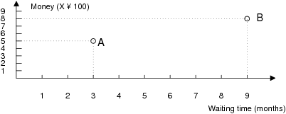
Figure 6: The adjusted money amount salient version for the scholarship problem in Experiment 3. 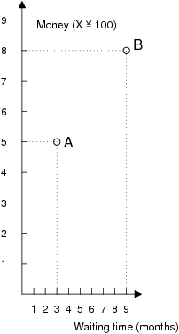
The Scholarship problem scenario employed by Experiment 1 was presented to participants. But Figures 1 and 2 were replaced by Figures 5 and 6, which now can be viewed and read as follows:
Please note that, in Figures 5 and 6, the scale resolution was kept constant while we manipulated the relative length perception salience of the attributes between the graph versions. Specifically, we graphed the attributes using 9 tic marks in both Figures 5 and 6. Any evaluation difference between the two graph versions thus cannot be attributed to the scale resolution. In addition, to eliminate the potential effect caused by the horizontal-vertical illusion, we counterbalanced the assignment of attributes to the axes. As a result, for the participants who were assigned to the waiting time salient version, about half of them saw the waiting time attribute on the X axis; whereas the other half saw this attribute on the Y axis. The same was true for the participants who were assigned to the money amount salient version.
The participants, who were randomly assigned to one of the two versions, were asked to rate the preference strength on a 9-point scale ranging from 1 (not at all) to 9 (extremely) for each type of scholarship. In the end, 104 participants responded to the waiting time salient version, and the other 107 participants responded to the money amount salient version. Thus, this is a 2 (scholarship type: type A vs. type B) × 2 (graph version: the waiting time salient version vs. the money amount salient version) mixed experimental design, with the graph version as the between-subjects factor and the scholarship type as the within-subjects factor. The dependent variable was the preference strength for a scholarship.
After rating the preference strength for the scholarship, each participant indicated the relative importance of the two attributes on a 9-point scale ranging from 10 (time is more important than money) to 90 (money is more important than time), and the relative normality of the way the figure was shown on a 9-point scale ranging from 10 (very abnormal) to 90 (very normal). We used 10/90 rather than 1/9 on the scale to avoid the possibility that students would simply copy their previous operation.
A 2×2 ANOVA on preference strength revealed that the main effect was significant for scholarship type, F(1, 209) = 17.744, p < .01. As we predicted, the ANOVA also showed a significant interaction between scholarship type and graph version, F(1, 209) = 4.482, p < .05, indicating that the effect of scholarship type on preference strength was influenced by the graph version. Specifically, type B (M = 6.925, N=107) was preferred over type A (M = 5.851, N=107) in the money amount salient version, t(106) = -4.105, p < .01. However, the relative preference of type B (M = 6.529, N=104) over type A (M = 6.173, N=104) was non-significant in the waiting time salient version, t(103) = -1.657, p > .05. These results were consistent with our Experiment 1 and thus ruled out the possibility that scale resolution caused the preference difference between the figures. Differences in the assignment of attributes to the two axes did not cause preference difference either for type A (t(102) = -0.795, p > .05) or for type B (t(102) = -0.789, p > .05) in the waiting time salient version; the same was true in the money amount salient version (for type A, t(105) = 0.112, p > .05; for type B, t(105) = -0.103, p > .05).
The results turned out to be inconsistent with our expectations in that they were not friendly to the attribute importance hypothesis. In our case, a higher relative importance score meant that the money attribute was regarded as more important than the time attribute. According to the importance hypothesis, the relative importance score should be higher in the money amount salient version than in the waiting time salient version. However the difference in the rated importance score between the waiting time salient version (M=68.558, N=104) and the money amount salient version (M=64.579, N=107) was not significant, t(209) = 1.522, p > .05.
To determine the normality of the figure equivalence between the two figure types (i.e., longer X axis vs. longer Y axis), we carried out a t-test. The result was that no significant difference was found between the participants who responded to the longer X axis figure (M = 45.048, N=105) and those who responded to the longer Y axis figure (M = 48.679, N=106), t(209) = -1.126, p > .05. This result thus showed that our two figure types were equally normal to our participants.
Preferences are often influenced by the description of the options (Tversky & Kahneman, 1981), the method of preference elicitation (Lichtenstein, & Slovic, 1971; Hsee, 1996; Shafir, 1993), and the choice context (Kahneman, Fredrickson, Schreiber, & Redelmeier, 1993; Berger, Meredith, & Wheeler, 2008; McCormick & McElroy, 2009). The present study also demonstrated a violation of descriptive invariance by manipulating the spatial representation of the options. Specifically, the relative graphical distance along an axis of the options of a given attribute was changed, causing the apparent salient aspect of the information to differ in its spatial representation as a function of the scale employed. The results of our Experiment 1 showed that scale manipulation had a significant impact on the evaluation. Experiment 2 repeated the scale manipulation effect in a different scenario and extended it to a multi-options context. By disentangling the effect of scale distance manipulation from the other variables (e.g., scale resolution and assignment of attributes to axes), Experiment 3 further supported the finding that the relative distance between options could affect the preference. While the proverb tells us that a picture can be worth a thousand words, our results showed that graphs may be manipulated to cause very different impressions of the same data.
The problem that remained after the first two experiments was why attribute salience in graphical representations induces evaluation bias. In Experiment 3, we investigated the importance hypothesis, but our evidence did not indicate that the participants regarded the longer axis as the more important attribute. Consequently, attribute importance could not be responsible for the preference difference between the graph versions. Perhaps our finding can be understood by analyzing the impact of visual processing on decision making. Researchers generally accept that visual processing takes place in two successive stages and is influenced by both sensory input and cognitive knowledge (Hoffman, 1978). The first stage, driven by sensory features (e.g., color, size), is thought to be automatic and preattentive. Thus the processing in the first stage can not be captured consciously. In the second stage, the information is affected by prior cognitive knowledge, enters the consciousness, and is acquired. Hoffman (1978) argued that the physical salience of items in the visual field is a critical variable determining which items are attended to and acquired during the second stage. In our case, the participants’ attention seems to have been attracted by the attribute with more salient physical feature (e.g., the longer distance between options) in the visual field, and the other attribute tended to be relatively ignored in the subsequent evaluation. Indeed, Tversky, Sattath and Slovic (1998) reported that individuals tend to concentrate on the most prominent attribute of two alternatives in choice situations. Note, however, that the impact of the physical feature on visual processing does not enter the consciousness, according to Hoffman. Thus, when the participants were asked to rate the attribute importance in an explicit way in our Experiment 3, no significant difference appeared between the two graph versions.
This inference is also consistent with current two-system theories. Researchers in judgment and decision making have advocated that human behavior reflects the operation of two distinct cognitive systems: a heuristic system and a controlled analytic system (Kahneman & Frederick, 2002; Stanovich & West, 2000). The heuristic system is a relatively effortless system that relies on intuitive perception; the analytic system is a slower, effortful, rule-based one. These two systems interact in a complex manner and appear to be competing to control behavior. From this two system perspective, although the analytic system should be insensitive to the physical features in a figure, the attribute salience in graphical representations would be related to intuitive perception and thus would affect the heuristic system. The heuristic system is the one that contributes to the differences in preferences between graph versions in our study. Interestingly, the two-system theory also held that natural assessments (e.g., size, distance) are unconsciously and automatically registered by the heuristic system. Researchers in this field can, therefore, hope that taking the two systems theory into account in future research will further our understanding of how manipulating scale influences evaluations in a graphical context. They could test whether the scale manipulation effect observed in this study will vary as a function of the operation of the two systems. For example, will the effect disappear when inhibiting the heuristic system or when strengthening the analytic system?
In addition, the selection of scale in graphs often seems to be regarded as unimportant when presenting information in real life. However, this is not wise, as our research shows that people’s preferences can be constructed rather than revealed in a graphical context. Thus a practical implication of this study will be to carefully consider the implications of the application of scale (de)compression in businesses such as advertising, financial reporting, investment programs, market analysis and sales.
Armstrong, L., & Marks, L. E. (1997). Stimulus context, perceived length, and the horizontal–vertical illusion. Perception & Psychophysics, 59, 1200–1213.
Attneave, F., & Block, G. (1974). The time required to compare extents in various orientations. Perception & Psychophysics. 16, 431–436.
Berger, J., Meredith, M. & Wheeler, S. C. (2008). Contextual priming: Where people vote affect how they vote. Proceedings of National Academy of Science, 105, 8846–8849.
Gattis, M., & Holyoak, K. J. (1996). Mapping conceptual to spatial relations in visual reasoning. Journal of Experimental Psychology: Learning, Memory, and Cognition, 22, 231–239.
Hoffman, J. E. (1978). Search through a Sequentially Presented Visual Display. Perception and Psychophysics, 23, 1–11.
Hsee, C. K. (1996). The evaluability hypothesis: An explanation for preference-reversal between joint and separate evaluations of alternatives. Organizational Behavior and Human Decision Processes, 67, 247–257.
Jarvenpaa, S. L. (1990). Graphic displays in decision making: The visual salience effect. Journal of Behavioral Decision Making, 3, 247–262.
Jones, S. K., Frisch, D., Yurak, T. J., & Kim, E. (1998). Choices and opportunities: Another effect of framing on decisions. Journal of Behavioral Decision Making, 11, 211–226.
Kahneman, D., & Frederick, S. (2002). Representativeness revisited: attribute substitution in intuitive judgment. Cambridge, UK: Cambridge Univ. Press
Kahneman, D., & Tversky, A. (1984). Choice, values, and frames. American Psychologist, 39, 341–350.
Kahneman, D., Fredrickson, B.L., Schreiber, C.A., & Redelmeier, D.A. (1993). When more pain is preferred to less: Adding a better end. Psychological Science, 4, 401–405.
Krider, R. E., Raghubir, P., & Krishna, A. (2001). Pizzas: Pi or Squared? Psychophysical Biases in Area Comparisons. Marketing Science, 20, 405–25.
Levin, I. P, & Gaeth, G. J. (1988). How consumers are affected by the framing of attribute information before and after consuming the product. Journal of Consumer Research, 15, 374–378.
Levin, I. P. (1987). Associative effects of information framing. Bulletin of the Psychonomic Society, 25, 85–86.
Li, S., Su, Y. & Sun, Y. (2010). The effect of pseudo-immediacy on intertemporal choices. Journal of Risk Research, doi:10.1080/13669870903551704
Lichtenstein, S., & Slovic, P. (1971). Reversal of preference between bids and choices in gambling decision. Journal of Experimental Psychology, 89, 46–55.
McCormick, M., & McElroy, T. (2009). Healthy choices in context: How contextual cues can influence the persuasiveness of framed health messages. Judgment and Decision Making, 4, 248–255.
Piaget, J. (1968). Quantification, conservation and nativism. Science, 162, 976–79.
Raghubir, P., & Das, S. R. (2010), The long and short of it: Why are stocks with shorter runs preferred? Journal of Consumer Research, 36, 964–982.
Raghubir, P., & Greenleaf, E. (2006). Ratios in proportion: What should be the shape of the package? Journal of Marketing, 70, 95–107.
Raghubir, P., & Krishna, A. (1996). As the crow flies: Bias in consumers’ map-based distance judgments. Journal of Consumer Research, 23, 26–39.
Raghubir, P., & Krishna, A. (1999), Vital dimensions: Biases in volume estimates. Journal of Marketing Research, 36, 313–26.
Shafir, E. (1993). Choosing versus rejecting: Why some options are both better and worse than others. Memory & Cognition, 21, 546–556.
Stanovich, K. E., & West, R. F. (2000). Individual differences in reasoning: Implications for the rationality debate. Behavioral & Brain Sciences, 23, 645-726.
Tversky, A., & Kahneman, D. (1981). The framing of decisions and the psychology of choice. Science, 211, 453–458.
Tversky, A., Sattath, S., & Slovic, P. (1988). Contingent weighting in judgment and choice. Psychological Review, 95, 371–384.
Tversy, A., Slovic, P., & Kahneman, D. (1990). The causes of preference reversal. American Economic Review, 80, 204–217.
Verge, C. G., & Bogartz, R. S. (1978). A Functional measurement analysis of the development of dimensional coordination in children. Journal of Experimental Child Psychology, 25, 337–53.
This document was translated from LATEX by HEVEA.