Judgment and Decision Making, vol. 5, no. 7, December 2010, pp. 467-476

Overprecision is the most robust type of overconfidence. We present a new method that significantly reduces this bias and offers insight into its underlying cause. In three experiments, overprecision was significantly reduced by forcing participants to consider all possible outcomes of an event. Each participant was presented with the entire range of possible outcomes divided into intervals, and estimated each interval’s likelihood of including the true answer. The superiority of this Subjective Probability Interval Estimate (SPIES) method is robust to range widths and interval grain sizes. Its carryover effects are observed even in subsequent estimates made using the conventional, 90% confidence interval method: judges who first made SPIES judgments considered a broader range of values in subsequent conventional interval estimates as well.

Keywords: overconfidence, overprecision, subjective probability, interval estimates, judgment and decision making.

1  Introduction

The Federal Home Loan Mortgage Corporation, otherwise known as Freddie Mac, provides an online calculator on its website (www.freddiemac.com) to help potential clients determine whether they should buy a home or rent one. Among the factors included in this calculation is the estimated appreciation value of the home in question, defined by the website as “the yearly percentage rate that an asset increases in value”. The user has to enter a percentage value by which, according to her best judgment, her potential home will increase or decrease. However, when a negative value (i.e., a forecast that the house’s value will go down) was entered, it was followed by an error message: “Please fix the following errors: Appreciation rate must be a number between 0.00 and 100.00.” The design of this online calculator conveyed Freddie Mac’s belief that housing prices can change only between 0% and +100%, with any rate outside this range being improbable. However, according to the Federal Housing Finance Agency (2010), the average yearly appreciation rate of houses in the United States was consistently outside this range from the second quarter of 2007 through the first quarter of 2010, falling as low as −12.03% (and even lower than −28% in some states). This forecasting error, among others, resulted in Freddie Mac’s near failure, before its take-over by the U.S. government in 2008. (More than two years later, in December 2010, Freddie Mac finally changed its on-line calculator to account for house value depreciation.)

The failure of Freddie Mac to anticipate a depreciation of U.S. house prices is but one of many examples of overprecision in judgment. Overprecision is a form of overconfidence, found to be both prevalent and particularly impervious to debiasing (Moore & Healy, 2008). Also referred to as overconfidence in interval estimates (e.g., Soll & Klayman, 2004), overprecision is the excessive certainty that one knows the truth. Among its documented consequences are errors in clinical diagnosis (Christensen-Szalanski & Bushyhead, 1981; Oskamp, 1965), excessive market trading (Daniel, Hirshleifer, & Subrahmanyam, 1998; Odean, 1999), and excessive conviction by individual climate scientists that they know the future trajectory of climate change (Morgan & Keith, 1995; Zickfeld, Morgan, Frame, & Keith, 2010). Overprecision is typically measured by eliciting a confidence interval — a range of values that the judge is confident, to a certain degree, will include the true value in question (Alpert & Raiffa, 1982). Research has repeatedly found that the confidence people have in their beliefs exceeds their accuracy, meaning that the confidence intervals they produce are too narrow (i.e., overly precise, see Soll & Klayman, 2004). This pattern is observed in novice as well as expert judgments (Clemen, 2001; Henrion & Fischhoff, 1986; Juslin, Winman, & Hansson, 2007; McKenzie, Liersch, & Yaniv, 2008; Morgan & Keith, 2008).

Attempts to debias overprecision have had limited success. Koriat, Lichtenstein, and Fischhoff (1980) argued that people’s excessive confidence in their beliefs is driven by the more extensive search they conduct for supporting evidence than for evidence that contradicts their beliefs. In their experiments, participants were presented with two possible answers to a question, chose the answer they thought was correct, and reported their confidence in the accuracy of their chosen answer. They were grossly overconfident when they expressed very high confidence. However, when asked to consider evidence contradicting their answers before reporting their confidence, participants reported lower confidence levels. Soll and Klayman (2004) manipulated this search for evidence by asking their participants to specify the fractile cutoffs at the top and bottom ends of the range of possible values. So instead of asking their participants to specify the ends of an 80% confidence interval, they asked their participants (1) for a number low enough that there was a 90% chance the true answer was above it; and (2) for a number so high that there was a 90% chance the true answer was below it. Using this approach, Soll and Klayman were able to modestly reduce overprecision.

Other research has tried to reduce overconfidence by focusing on the format of the question (Juslin, Wennerholm, & Olsson, 1999; Seaver, von Winterfeldt, & Edwards, 1978; Teigen & Jørgensen, 2005). This research found that interval evaluation, based on probability judgments of fixed intervals, produces less overconfidence than interval production. For example, participants asked to create 90% confidence intervals produce excessively-narrow intervals, but other participants, who subsequently estimate their confidence for the participant-created intervals, report less than 90% confidence in their accuracy. Building on these findings, Winman, Hansson, & Juslin (2004) proposed the adaptive interval assessment (ADINA) method of eliciting judgments. Using this method, a desired confidence level for an interval is determined in advance. An interval is produced around a specific value (generated either by the judge, a peer, or at random), and the judge estimates the probability that this interval contains the correct answer. If this probability is higher than the desired confidence level, a narrower interval is presented next, and, similarly, if the initial probability is lower than the desired probability, then a wider interval is presented. This procedure is repeated until the probability assigned to the interval matches the desired confidence level. The authors found that the resulting intervals from this procedure displayed less overprecision than intervals that were produced directly. Unfortunately, this reduction in overprecision appeared to be tied to the assessment format: subsequent assessments made with a different response format (e.g., confidence intervals) reverted to their old, overly precise form, suggesting that the change in methods did not affect the cognitive process by which estimates were produced. In short, no method has been found that both reduces overprecision and trains judges to consider a wider range of values when making subsequent estimates in a different format.

1.1  SPIES - Subjective Probability Interval Estimates

We propose a novel method of producing interval estimates for quantitative values that has the potential to significantly reduce overprecision. Our method, Subjective Probability Interval Estimates (SPIES), works by forcing judges to consider the entire range of possible answers to a question. The judge sees the full range of possible outcomes, divided into a series of intervals. For each interval, the judge estimates the probability that it includes the correct answer, with the sum of these probabilities constrained to equal 100% (e.g., Figure 1).

---

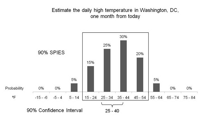
Figure 1: Illustration of hypothetical estimates using SPIES and a 90% confidence interval for the daily high temperature in Washington, DC, one month in the future. The 90% SPIES interval ranges from 15ºF to 54ºF, whereas the 90% confidence interval ranges from 25ºF to 40ºF.

---

We expect SPIES will be superior to previously instantiated methods for two reasons. First, SPIES forces judges to consider all possible values, including extreme values, which they may otherwise fail to consider spontaneously. Overlooking these extreme values may account, at least in part, for the overprecision observed in interval estimates. By requiring the judge to consider all values and assign each of them some probability of being correct, even if this probability is zero, SPIES may significantly reduce this bias.

Second, the SPIES method includes features found to be instrumental in reducing overprecision. This method makes use of multiple judgments, which, as Soll & Klayman (2004) found, produce lower overprecision than single interval estimates. Also, building on the findings of research on format dependence (e.g., Juslin et al., 2007; Teigen & Jørgensen, 2005), SPIES is based on probability judgments, which appear to induce less overprecision than do interval estimates. This reduction may be further enhanced by constraining the summed probability assigned to outcomes to equal 100%, limiting the tendency to overstate subjective probabilities (Tversky & Koehler, 1994).

We report three experiments that tested our approach. Experiment 1 compared overprecision levels produced by SPIES to those produced by other methods of eliciting quantitative predictions. Experiment 2 tested the robustness of SPIES to different range widths and interval grain sizes. Experiment 3 tested the robustness of SPIES to ranges with defined bounds, and examined whether SPIES can increase accuracy of estimates of extreme values, as well as of values which lay closer to the middle of the range. In addition, Experiment 3 measured the carryover effects of SPIES on subsequent estimates made using a different method.

2  Experiment 1

Experiment 1 tested whether SPIES can reduce overprecision, relative to two other methods of estimating intervals — 90% confidence intervals, the most widely used method of interval production, and 5^th and 95^th fractile estimates, which together imply a 90% confidence interval.

2.1  Method

2.1.1  Participants

103 Pittsburgh residents responded to an email solicitation, sent to past participants in studies of the Center for Behavioral Decision Research, inviting them to participate in an online study. One of the participants was randomly selected to receive a $100 prize.

2.1.2  Procedure

Participants estimated the high temperature in Pittsburgh one month from the day on which they completed the survey, in three different formats. In a 90% confidence interval format, participants entered two values, between which they were 90% sure the actual temperature would fall. In a fractile format, participants specified their estimated distribution’s 5^th fractile (i.e., a number sufficiently low that they were 95% sure it would be below that the actual temperature), and the 95^th fractile (i.e., a number they were 95% sure would fall above the actual temperature). In addition, participants made Subjective Probability Interval Estimates (SPIES) — they were presented with the following temperature intervals: below 40°F, 40–49, 50–59, 60–69, 70–79, 80–89, 90–99, 100–109, and 110°F or above. They then estimated, for each interval, the probability that it would contain the actual temperature. The web page required the participants to adjust the probabilities so that they summed to 100% before proceeding. Presentation order of the three formats was randomly determined, and not recorded.

2.2  Results

Because the assigned confidence level for intervals produced by the first two methods was 90%, we chose this level as our target confidence for intervals produced by SPIES. We used an algorithm to calculate these confidence intervals, which identifies the temperature interval with the highest subjective probability and adds its neighboring intervals until the sum of probabilities reaches closest to, but not more than 90%. The algorithm then adds the proportion of the adjacent interval with the next highest probability (or the two intervals on both sides of the aggregated interval, when they are assigned equal probabilities) needed to reach 90%. We refer to the resulting confidence interval as 90% SPIES.¹ This is a conservative calculation of 90% SPIES, designed to produce a confidence interval out of the fewest possible subjective probability intervals. In cases where an extreme interval (i.e., below 40°F, 110°F or above) was included in a participant’s 90% SPIES, we calculated that interval’s width as 10°F.

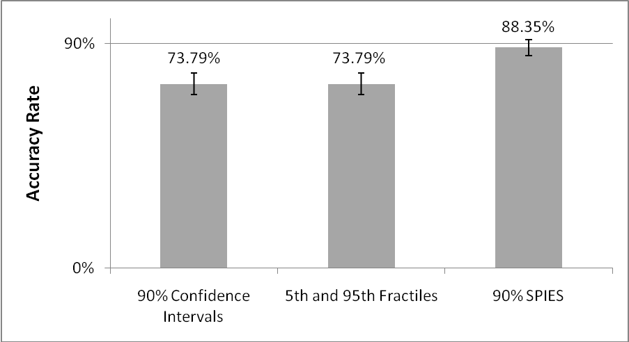
The true temperatures on the days for which participants made their estimates were between 67°F and 73°F. A repeated-measures ANOVA comparing the accuracy of participants’ estimates across the three methods revealed a significant difference, F(2, 101) = 4.98, p = .009, η ² = .090. 90% confidence intervals and intervals produced by the 5^th and 95^th fractiles did not differ in their accuracy, both including the correct answer 73.79% of the time (SD = 44.19).² 90% SPIES, however, included the correct answer in 88.35% of the estimates (SD = 32.24), a significantly higher hit rate than both 90% confidence intervals, t(102) = 2.88, p = .005, d = 0.57, and fractiles, t(102) = 2.69, p = .008, d = 0.53. Whereas 90% confidence intervals and fractiles displayed significant overprecision of 16.21%, ts(102) = 3.72, p < .0005, d = 0.74, the accuracy level produced by SPIES was not significantly different from the 90% confidence level assigned to them, t(102) = 0.52, p = .60, meaning that these estimates did not exhibit overprecision (see Figure 2).

---

Figure 2: Accuracy rates displayed by 90% confidence intervals, fractiles and 90% SPIES in Experiment 1. Error bars indicate ±1 SE.

---

The SPIES method does not seem to have improved participants’ intuition regarding the precise temperature, as measured by the distance between an interval’s midpoint and the true answer. A repeated-measures ANOVA revealed a significant method effect, F(2, 101) = 3.49, p = .034, η ² = .065, but the midpoints of 90% SPIES intervals were not significantly closer to the true answer than either those of 90% confidence intervals, t(102) = 1.39, p = .167, or those between the 5^th and 95^th fractiles, t < 1.

We also compared the widths of the intervals generated by the three methods. A repeated-measures ANOVA revealed a significant effect of method on interval width, F(2,101) = 21.71, p < .0005, η ² = .301. Within-subject contrasts show that 90% SPIES intervals were significantly wider (M = 31.81, SD = 11.96) than 90% confidence intervals (M = 23.58, SD = 14.42), t(102) = 5.73, p < .0005, d = 0.62, but slightly, and non-significantly, narrower than fractiles (M = 33.15, SD = 22.48), t < 1. The fractile estimates’ relatively large mean width, as well as their high variability, can be accounted for by the fact that eight of these estimates reached either below 30°F or above 119°F (the boundary values we set for calculating 90% SPIES), and resulted in relatively wide intervals.³

2.3  Discussion

Of the three methods tested in this experiment, the SPIES method was the only one in which confidence was correctly calibrated with accuracy. Although 90% confidence intervals and fractile estimates produced a higher hit rate than that typically found in prior research (Klayman, Soll, Gonzalez-Vallejo, & Barlas, 1999), the accuracy of SPIES was significantly higher than both of these methods. Moreover, the SPIES method not only produced better accuracy, it eliminated overprecision.

Another noteworthy finding is that SPIES produced a significantly higher hit rate than did fractile estimates. This result suggests that, although in both methods judges unpack their estimates into multiple judgments, this feature is not the primary driver of the superior calibration found in SPIES.

The results of this experiment are not conclusive regarding why SPIES were more accurate. On the one hand, interval midpoints did not differ between the three estimation formats in their distance from the true value, suggesting the better hit-rate is due to the estimates made using SPIES being more inclusive. On the other hand, 90% SPIES achieved a higher hit rate than fractile estimates without being significantly wider. As noted, we believe this is due to the constraint put on including extreme values in the SPIES intervals, but not in the other estimates. This issue was addressed in Experiment 3. First, we wanted to test whether the improved performance produced by SPIES holds for different configurations of intervals. This is an important issue because the SPIES method necessitates two choices: how big to make the range of possible responses and into how many intervals to divide that range. These variations may influence the amount of attention given by the judge to the values she considers, and, subsequently, affect the quality of the estimates produced. Therefore, we sought to test the robustness of the results obtained in Experiment 1 to these variations.

3  Experiment 2

In Experiment 2, we varied the width of the range of subjective probability intervals for which estimates were made and the number of intervals into which this range was divided. We expected that SPIES would be better calibrated than 90% confidence intervals, regardless of the width of their range, or of how many intervals the SPIES task consisted.

3.1  Method

3.1.1  Participants

The study was conducted online, using participants from Amazon Mechanical Turk (described by Paolacci et al., 2010). 116 U.S.-based participants (63 women, M_age = 36.78) completed a survey for 5¢ each.

3.2  Procedure

Participants estimated the day’s high temperature in Washington, DC exactly one month after the day on which they took the survey. In a 2 x 2 between-subjects design, participants specified SPIES intervals with a narrow range (−15°F to 84°F)⁴ or with a wide range (−65°F to 134°F), which were divided into either ten or twenty intervals. These divisions resulted in three interval grain-sizes: fine (5°F), medium (10°F) and coarse (20°F). Two intervals of extreme values were added at both ends of these ranges: “-16°F or lower” or “-166°F or lower” at one end, and “85°F or higher” or “135°F or higher” at another end (see Table 1). To compare SPIES with conventional interval estimates, an additional group of participants produced a 90% confidence interval.

3.3  Results

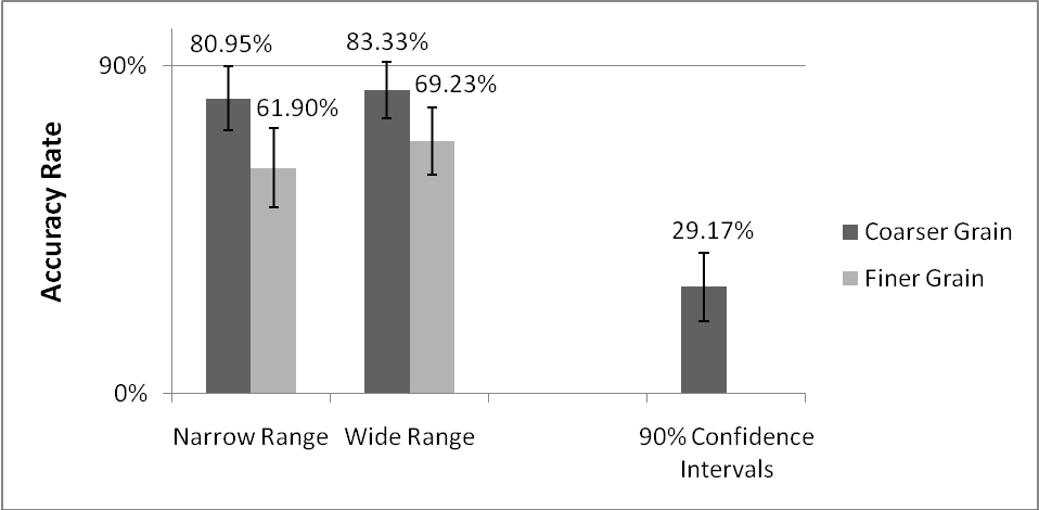
Actual temperatures on the days for which participants provided their estimates fell between 31°F and 40°F. First, we compared the accuracy of 90% confidence intervals to that of estimates made using SPIES. Similar to Experiment 1, 90% SPIES achieved a significantly higher hit rate (M = 73.91%, SD = 44.15) than 90% confidence intervals (M = 29.17%, SD = 46.43), t(114) = 4.38, p < .0005, d = 0.99. As expected, 90% SPIES of all four configurations produced accurate estimates at a significantly higher rate than 90% confidence intervals, ts ≥ 2.28, ps ≤ .027, ds ≥ 0.68 (see Figure 3).

---

Figure 3: Accuracy rates displayed by SPIES of different range widths and grain sizes and by 90% confidence intervals in Experiment 2. Error bars indicate ±1 SE. See Table 2 for hit rates of the different SPIES configurations.

---

Second, we tested whether the different configurations of the SPIES task affected participants’ estimates. A 2 (range width: 100°F, 200°F) x 2 (number of intervals: 10, 20) between-subjects ANOVA on the hit rates of 90% SPIES revealed no significant effects of either range width, F < 1, or number of intervals, F(1,88) = 3.23, p = .08; nor was there a significant interaction, F < 1 (see Table 2). In order to perform a more conservative test of the effect of range width on participants’ estimates, we compared the two conditions in which participants made SPIES judgments with a medium, 10ºF grain size (see Table 1). These two conditions differed only in range width: one group was presented with a 100ºF range, whereas for the other group, the SPIES task spanned 200ºF. The comparison between these two groups revealed no significant effect of range width on hit rates (100ºF range: M = 80.95%, SD = 40.24%; 200ºF range: M = 69.23%, SD =47.07%), t < 1.

---

Table 1: Range Width and Grain Size Condition Assignment in Experiment 2.

Range Width	Number of intervals	Grain Size	Extreme Intervals
Narrow (100ºF)	20 + 2 extreme intervals	Fine (5ºF)	−16°F or lower 85°F or higher
Narrow (100ºF)	10 + 2 extreme intervals	Medium (10ºF)	−16°F or lower 85°F or higher
Wide (200ºF)	20 + 2 extreme intervals	Medium (10ºF)	−66°F or lower 135°F or higher
Wide (200ºF)	10 + 2 extreme intervals	Coarse (20ºF)	−66°F or lower 135°F or higher

---

We did, however, find that the width of 90% SPIES was affected by the configuration of the task. We conducted a similar ANOVA on estimate width, which revealed significant main effects of the overall SPIES’ range width and the number of intervals it included, F(1,88) = 12.52, p = .001, η ² =.125 and F(1,88) = 12.25, p = .001, η ² =.122, respectively, with no interaction, F < 1 (see Table 3). However, a comparison of the two 10ºF grain size groups found no effect of range width on estimate width (100ºF range: M = 33.40, SD = 16.58; 200ºF range: M = 33.50, SD = 12.93), t < 1.

As in Experiment 1, the estimated intervals’ midpoints were not affected by our manipulations. The distances of 90% SPIES’ midpoints from their respective true values did not vary with range width, F(1, 88) = 1.47, p = .228, or with grain size, F < 1, nor was there an interaction, F < 1. No significant difference in midpoint accuracy was found between 90% SPIES and 90% confidence intervals, either, t < 1.

In light of the significant effects on estimate width and the large, though only marginally-significant effect of number of intervals on hit rates, we sought to examine the extent to which participants were sensitive to the different SPIES configurations. We tested this by measuring the number of intervals to which participants assigned some probability higher than zero in their estimates. A 2 (range width) x 2 (number of intervals) ANOVA found a significant effect of interval number, wherein participants for whom the SPIES task consisted of twenty intervals gave significantly more intervals (M = 6.36, SD = 3.81) non-zero probabilities than those who were presented with only ten intervals (M = 4.24, SD = 2.30), F(1, 88) = 14.94, p < .0005. The ANOVA also found a significant range width effect, F(1, 88) = 22.69, p < .0005, but the direct comparison of the two 10ºF grain size groups found no effect of range width on the number of intervals with non-zero probabilities (100ºF range: M = 5.14, SD = 2.83; 200ºF range: M = 4.62, SD = 1.79), t < 1. Together, these results suggest that participants who made estimates with the finer-grained SPIES were aware of the need to use a larger number of intervals and adjusted their estimates, but not sufficiently to fully equate their estimates’ width to those made with coarser-grained intervals.

---

Table 2: 90% SPIES hit rates by range width and grain size in Experiment 2.

	Range Width
Number of intervals	Narrow	Wide
10	80.95% (40.24%)	83.33% (38.07%)
20	61.90% (49.76%)	69.23% (47.07%)

---

---

Table 3: 90% SPIES width (in degrees F) by range width and grain size in Experiment 2.

	Range Width
Number of intervals	Narrow	Wide
10	33.40 (16.58)	44.95 (11.80)
20	25.48 (11.12)	33.50 (12.93)

---

3.4  Discussion

As in Experiment 1, SPIES had a significantly higher hit rate than standard 90% confidence interval estimates. More important, this difference was consistent across the various range widths and interval grains.

One common feature of the first two experiments is that both included estimates of values on an unbounded scale (i.e., temperatures), for which we did not specify a minimum or a maximum value. In the absence of such explicit bounds, the highest and lowest intervals in the SPIES task may be perceived by the judge as reasonable bounds, between which the experimenters expect the true answer to lie. Because these intervals were included in the SPIES tasks, but not in confidence interval estimates, they may account for some of the difference in performance between the two methods. Also, in both experiments, the true values eventually fell closer to the middle of the scale than to any one of its ends. In Experiment 3 we sought to address these issues, by specifying the high and low bounds of the range in all conditions, as well as by varying the true values being estimated.

Another question which remains open is whether the difference between SPIES and confidence interval production is solely due to the different elicitation format, or whether SPIES enact a change in the underlying process by which estimates are generated. We hypothesize that training judges to consider the entire range of possible values, using SPIES, will have effects beyond the current elicitation method, and will affect subsequent estimates made in different formats. We tested this hypothesis in Experiment 3.

4  Experiment 3

In Experiment 3, participants estimated a series of values, using confidence intervals for half of their estimates and SPIES for the others. Participants estimated the year in which all 20^th Century U.S. presidents were first elected to office. These years were therefore on a bounded scale, ranging from 1900 to 1999. In addition, since these election years for all presidents were estimated, the true values fell at various points on the scale, both near the ends and closer to the middle.

We varied the elicitation method within-subjects. Participants produced 90% confidence intervals for half of their estimates, and SPIES for the other half, the order of which was counterbalanced. This design enabled us to test for the influence of SPIES on subsequent confidence interval estimates, by measuring differences in 90% interval widths between confidence intervals produced before SPIES and those produced after. If format dependence is solely responsible for the reduction in overprecision exhibited in SPIES, then, similar to the findings of Winman et al. (2004), confidence intervals will not be affected after switching from SPIES. If, as we suggest, SPIES change the process by which judges make confidence estimates, then 90% confidence intervals should include a wider range of values if made after SPIES than when made beforehand.

4.1  Method

4.1.1  Participants

334 Pittsburghers (169 women, M age = 22.6, SD = 6.79) completed a survey in the lab, in exchange for $3 or course credit.

4.1.2  Procedure

Participants answered a 16-item quiz, estimating the years in which all 20^th Century U.S. presidents were first elected to office⁵. For each president, participants estimated either a 90% confidence interval or SPIES. The SPIES task included all years from 1900 to 1999, divided into ten intervals, each representing a decade, with no end intervals for more extreme values. Similarly, in the confidence interval production condition, any estimate that included years outside the 20^th century could not be submitted, and the participant was instructed to revise it. Half of the participants provided 90% confidence intervals for the first eight estimates and SPIES for the last eight; for the other half, this order was reversed. Items appeared in a different random order for each participant.

4.2  Results

We calculated 90% SPIES the same way as in Experiments 1 and 2. Next, we conducted a 2 (elicitation method: SPIES, confidence intervals) x 2 (elicitation order: first eight estimates, last eight estimates) mixed ANOVA⁶ on hit rates, which showed that 90% SPIES had a significantly higher hit rate than 90% confidence intervals. SPIES included the correct answer 76.91% of the time (SD = 20.17), compared with 54.34% (SD = 26.26%) in 90% confidence intervals, F(1,332) = 192.34, p < .001, η ² =.367. This result supported our prediction that SPIES would provide greater accuracy for estimated values in bounded ranges, regardless of where on the range the true value eventually falls. As in Experiments 1 and 2, we found no significant effect of elicitation method on interval midpoint accuracy, F(1, 332) = 1.11, p = .29.

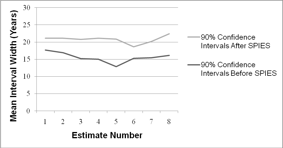
A similar ANOVA on estimate width yielded a significant effect of SPIES on subsequent confidence interval width. SPIES produced significantly wider estimates (M = 36.27, SD = 20.09) than 90% confidence intervals (M = 18.17, SD = 14.84), but there was also a significant Elicitation method x Elicitation order interaction, F(1,332) = 3.97, p = .047, η ²= .012. Simple effects tests revealed that 90% confidence intervals produced after having taken the SPIES task were significantly wider (M = 20.77 years, SD = 16.13) than those produced in the first set of estimates (M = 15.57, SD = 12.95), t(332) = 3.25, p = .001, d = 0.36, whereas 90% SPIES did not differ between the two groups, t < 1. This result suggests that SPIES had a carryover effect on subsequent confidence interval estimates, leading judges to consider a wider range of values in their estimates. To rule out learning and time effects, we conducted a repeated-measures ANOVA on confidence interval widths for each item participants estimated. The last confidence interval estimate in each set was not, on average, wider than the first estimate in the set, F < 1, suggesting the greater width of confidence intervals made after SPIES than of those made before SPIES was not due to a simple improvement with experience or time within the same elicitation method (see Figure 4).

---

Figure 4: Estimate-by-estimate mean widths of 90% confidence intervals made in the first set of estimates (before SPIES), compared to those of 90% confidence intervals in the second set of estimates, after having made SPIES judgments in the first set in Experiment 3.

---

4.3  Discussion

The results of this experiment confirm that the increased accuracy observed in SPIES does not depend on features of the possible range of values being estimated, or on where on this range the true value actually falls. Furthermore, the carryover effect of SPIES on subsequent confidence interval estimates suggests that the reduced bias in SPIES is not due to format dependence alone. It also demonstrates a change in the process by which judgments are made. The more extensive consideration of values in SPIES prompted judges to generate wider confidence intervals in later estimates.

5  General discussion

Overprecision in judgment continues to be a robust and intriguing phenomenon with potentially profound and harmful consequences in domains as diverse as corporate investment and scientific progress (e.g., Henrion & Fischhoff, 1986; Malmendier & Tate, 2005; Morgan & Keith, 2008). SPIES appears to be a practical and simple method of producing interval estimates that effectively reduces overprecision. Across three experiments that elicited different estimates, SPIES led to greater accuracy than other elicitation methods — and in some cases completely eliminated overprecision. The results further suggest that SPIES may affect the process by which people make quantitative estimates, as confidence interval estimates produced after SPIES included a wider range of values than estimates produced before this intervention.

Future research is needed to elucidate the underlying mechanism by which SPIES results in reduced overprecision. SPIES may evoke a more extensive search for information, which puts the judge in a more inquisitive mindset (e.g., Galinsky, Moskowitz, & Skurnik, 2000), leading to a better and more deliberate estimation process. Alternatively, considering all subjective probability intervals may work by increasing the amount of available estimate-relevant information in memory, forcing a fuller consideration of alternative hypotheses (Hirt & Markman, 1995; McKenzie, 1997, 1998; Morewedge & Kahneman, 2010).

In addition to our laboratory findings, we believe SPIES can easily be used for producing estimates in real-world settings. As Experiment 2 shows, SPIES provides superior results to confidence interval estimates, regardless of how the SPIES task is presented. The structure of the method, which utilizes the entire range of possible values, allows the production of intervals of virtually any target width or confidence level from the same estimate, and even allows changing the target width or confidence without having to estimate the same value multiple times. Furthermore, SPIES appears to have positive carryover effects, suggesting that the method may help train judges to improve their estimates when the range of possible outcomes of an event is uncertain and traditional confidence interval estimates are required.

Another useful feature of SPIES is the added information it provides about the judge’s sense of uncertainty regarding the estimated value. Traditional confidence intervals provide information only about the two values beyond which the judge thinks the true value has a very low chance of being, but not which values within the confidence interval are perceived as more probable than others. Point estimates and probability judgments, which are widely used in industry, provide very little information about the judge’s sense of the extent to which the true value may vary. SPIES, on the other hand, provides information on the values which the judge estimates as the most probable, as well as her sense of the variability in her estimate. This information can be highly valuable in cases such as estimates of future product demands which affect present stock, production and pricing.

One limitation of the experiments depicted in this paper is that they tested the SPIES method on only one type of estimates plagued by overprecision, namely interval estimates. Future research should test whether this method is applicable in forecasts of discrete events (e.g., the chances that a building will sustain an earthquake; which candidate will win an election). Another limitation is that, despite its simplicity for the judge, the SPIES method is too complex and time consuming for many everyday estimates. The use of SPIES is recommended in contexts where the consequences are large and ample time or a computer is available to calculate a confidence interval, but they are hardly the panacea for all estimates and forecasts. Nevertheless, we believe expert judges and professionals who make estimates of uncertain quantities may benefit from adopting SPIES.

References

Appendix: MATLAB code for calculating SPIES

%Your input data file should be in a .csv file, and include only the
%data entered in the SPIES task, without column headers or participant
%ID's. The output file will be a text file, which will include the
%subjective probabilities incorporated in the result interval, as well
%as the interval's low and high bounds.

function [] = SPIES(filename)
 filenamenew = [filename(1:(end - 4)) 'out.txt'];
 data = importdata(filename);

%The four lines below this comment are for configuring your SPIES task:
%rangeMin = the SPIES task's low bound.
%rangeMax = the SPIES task's high bound.
%intervalGrainSize = the width of the SPIES' intervals.
%targetConfidence = the result confidence interval's desired level of
%  confidence.
 rangeMin = 0;
 rangeMax = 100;
 intervalGrainSize = 10;
 targetConfidence = 90;
 
 minColRange = (rangeMin:intervalGrainSize:rangeMax - intervalGrainSize); 
 maxColRange = (rangeMin+intervalGrainSize:intervalGrainSize:rangeMax);
 result = [];
 for ii = 1:size(data, 1)
   dataRow = data(ii, :);
   len = length(dataRow);
   matrix = zeros(len, len);
   for i1 = 1:len
     for j1 = i1:len
       matrix(i1, j1) = sum(dataRow(i1:j1));
     end
   end
   maxValueIndex = 1;
   for k = 1:len
       if (dataRow(k) >= dataRow(maxValueIndex))
         maxValueIndex = k;
       end  
   end
   bottom = maxValueIndex;
   top = maxValueIndex;
   while (sum(dataRow(bottom:top)) <= targetConfidence)
       if (bottom > 1)
         if (top == len)
             bottom = bottom - 1;
         else
             if (dataRow(bottom - 1) > dataRow(top + 1)) 
                 bottom = bottom - 1;
             else
                 if (dataRow(bottom - 1) < dataRow(top + 1)) 
                  top = top + 1;
                 else
                   if (dataRow(bottom - 1) == dataRow(top + 1))
                       top = top + 1;
                       bottom = bottom - 1;
                   end
                 end
             end
         end
         else
         if (top < len)
             top = top + 1;
         else
             % This should not happen
         end 
       end
     end
   includedSPIES = zeros(1, len);
   includedSPIES(bottom:top) = dataRow(bottom:top);
   startRange = minColRange(bottom);
   endRange = maxColRange(top);    
   while (sum(includedSPIES(bottom:top)) > targetConfidence || ...
           includedSPIES(bottom) == 0 || includedSPIES(top) == 0 )
       extra = sum(dataRow(bottom:top)) - targetConfidence; 
       if (extra == 0)
         while (includedSPIES(bottom) == 0)
           bottom = bottom + 1; 
         end
         while (includedSPIES(top) == 0)
           top = top - 1; 
         end
           startRange = minColRange(bottom);
           endRange = maxColRange(top);
         continue;
       end
       if (dataRow(bottom) + dataRow(top) <= extra) 
         includedSPIES(bottom) = 0;
         includedSPIES(top) = 0;
         bottom = bottom + 1;
         top = top - 1;
         startRange = minColRange(bottom);
         endRange = maxColRange(top);
         continue;
       end  
       diff = dataRow(bottom) - dataRow(top);
       if (diff == 0)
         valuePerUnit = dataRow(bottom) / intervalGrainSize;
         unitToUse = dataRow(bottom) - (extra / 2);
         startRange = maxColRange(bottom) - ...
                   (unitToUse / valuePerUnit);
         endRange = minColRange(top) + ...
                  (unitToUse / valuePerUnit);
         includedSPIES(top) = includedSPIES(top) - (extra / 2);
         includedSPIES(bottom) = includedSPIES(bottom) - (extra / 2);
         continue;
       end
       if (diff > 0)
         if (dataRow(top) <= extra)
             includedSPIES(top) = 0;
             top = top - 1;
             endRange = maxColRange(top);
             continue;
         end
         valuePerUnit = dataRow(top) / intervalGrainSize;
         unitToUse = dataRow(top) - (extra);
         endRange = minColRange(top) + ...
                  (unitToUse / valuePerUnit);
         includedSPIES(top) = includedSPIES(top) - (extra);
         continue;          
       end
       if (diff < 0)
         if (dataRow(bottom) <= extra)
             includedSPIES(bottom) = 0;
             bottom = bottom + 1;
             startRange = minColRange(bottom);
             continue;
         end
         valuePerUnit = dataRow(bottom) / intervalGrainSize;
         unitToUse = dataRow(bottom) - (extra);
         startRange = maxColRange(bottom) - ...
                  (unitToUse / valuePerUnit);
         includedSPIES(bottom) = includedSPIES(bottom) - (extra);
         continue;  
       end
     end
   result(ii, 1:(len + 2)) = [includedSPIES,startRange, endRange];
 end
dlmwrite(filenamenew, result, ' ');

*

The authors wish to thank Nir Kerem, Dafna Shahaf and Lior Lipshitz for help in developing the SPIES calculation algorithm, and the staff and facilities of the Center for Behavioral Decision Research at CMU. Correspondence concerning this paper should be addressed to Uriel Haran, Tepper School of Business, Carnegie Mellon University, 5000 Forbes Avenue, Pittsburgh, PA, 15213, email: uharan@cmu.edu.

1

The full algorithm used to calculate 90% SPIES interval is in the Appendix.

2

The identical result for 90% confidence intervals and the fractile method appears to be coincidental, as 63 participants were accurate in both their 90% confidence intervals and fractile estimates, whereas 26 were accurate in only one of the two formats.

3

Only one 90% confidence interval exceeded these boundary values.

4

The highest and lowest temperatures, respectively, ever recorded in Washington, DC in February, the target month for participants’ forecasts..

5

We excluded William McKinley, who was first elected in 1896, and Gerald Ford, who was never elected president.

6

Since we counterbalanced elicitation order between the two groups (i.e., one group estimated SPIES intervals for the first eight estimates and confidence intervals for the last eight, whereas the other group made estimates in the reverse order), the group means are equal to the method x order interaction.

In formal terms, the group main effect is: H₀: (SPIES₁ + Conf. Int₂) – (Conf.Int₁ + SPIES₂) = SPIES₁ + Conf. Int₂ – Conf. Int₁ – SPIES₂ = 0.

The method x order interaction is: H₀: (SPIES₁ – SPIES₂) – (Conf. Int₁ — Conf. Int₂) = SPIES₁ – SPIES₂ – Conf. Int₁ + Conf. Int₂ = 0.

Note that these two equations are the same. Therefore, a difference in the estimates of the two groups would imply a significant interaction between the elicitation method and order (i.e., first eight estimates vs. last eight).

This document was translated from L^AT_EX by H^EV^EA.