Direct and indirect effects of pathological gambling on
risk attitudes
Pablo Brañas-Garza1
Universidad de Granada
Nikolaos Georgantzís
Universitat Jaume I
Pablo Guillen
University of Sydney
Judgment and Decision Making, vol. 2, no. 2, April 2007,
pp. 126-136.
Abstract
We study individual decision making in a lottery-choice task
performed by three different populations: gamblers under
psychological treatment (äddicts"), gamblers' spouses
("victims"), and people who are neither gamblers or gamblers'
spouses ("normals"). We find that addicts are willing to take
less risk than normals, but the difference is smaller as a
gambler's time under treatment increases. The large majority of
victims report themselves unwilling to take any risk at all.
However, addicts in the first year of treatment react more than
other addicts to the different values of the risk-return
parameter.
Keywords: risky decision making, pathological gambling,
attraction and repulsion to chance.
1 Introduction
Since the late 1940s, individual decision making under risk has been one of
the most popular issues studied by economists and psychologists. On one
hand, theoretical analysis, initially undertaken mostly by economists, has
framed the basic problem as a generic situation in which individuals choose
from a number of probability-outcome pairs. On the other hand, empirical
contributions from both disciplines have adopted a variety of methodologies.
These include questionnaires, economic experiments, and real-world data. The
most salient and intriguing result across all these different methodologies
is that decisions in a risky environment are very sensitive to the framing
of the choice task and to some individual characteristics. In this paper, we
focus on the effects of problem gambling on individual choice under
uncertainty, as a natural field for studying interaction between subjects'
characteristics and their observed decision making behavior.
Since 1980, pathological gambling has been included in the
Diagnostic and Statistical Manual of Mental Disorders published
by the American Psychiatric Association (1980). Patients with
spectrum-related disorders show an intense desire to perform a
specific behavior preceded by unpleasant feelings and
physiological activation, all of which are relieved when the
behavior is performed (Cartwright et al., 1998). Thus, several
authors consider pathological gambling (PG) as an
obsessive-compulsive spectrum disorder (Frost, 2001 ). Contrary
to this view, other authors argue that gambling is essentially
egosyntonic for the patients in all phases of the disorder, in
contrast to what happens in the obsessive-compulsive spectrum
disorders, where the behavior is consistently egodystonic
(American Psychiatric Association, 1994). Moreover, compulsive
behaviors include increased evasive behavior, anticipatory
anxiety and risk aversion, which are not usually observed in the
behavior of pathological gamblers (PGs).
This lack of agreement among experts on whether gambling is an egosyntonic
or egodystonic disorder could even imply that gamblers may be heterogeneous
with respect to their attitudes towards their addiction. Therefore, at a
first stage, whether gambling is an egosyntonic or egodystonic disorder
would influence the way PGs feel about their condition. At a second stage,
this could interfere with the degree to which they feel more attracted than
normal subjects by bets involving riskier options. Therefore, studying
whether PGs behave differently from normal subjects in risky decision-making
tasks would require isolating the first level of pleasure or discomfort due
to being a gambler from the second level of pleasure due to betting on
riskier options. A natural way of obtaining a more homogeneous population of
gamblers with respect to their attitude towards their addiction is isolating
and studying a population of egodystonic gamblers as are those who have
voluntarily decided to quit and participate in a Gambler Anonymous (GA)
therapy group.
Several aspects of PGs' behavior have been studied so far. Such studies are
either aimed at shedding light on specific methodological issues that should
be accounted for when studying decision making by PGs2 or are
directly addressing the question whether PGs suffer form some kind of
cognitive bias. Among different kinds of cognitive bias, the most obvious
suspect is probability distortion due to attraction to risky bets, which
could yield irrational behavior reflected on higher degrees of risk taking
as compared to normal subjects. Along this line are the studies by Toneatto
(1999a,b), Gaboury and Ladouceur (1989)
and, especially, Leopard (1978), while Goodie (2005) adopts a
slightly different approach to higher levels of risk taking showing that
they are the result of overconfidence.
In this paper, we study risky decisions made by subjects whose lives have
been directly affected by pathological gambling and have decided to quit by
participating in a therapy group of GA. Furthermore, we study the risk
taking behavior of people who are indirectly affected by pathological
gambling because they are married to a pathological gambler. We want to know
whether the decisions of the aforementioned groups in an abstract
lottery-choice task significantly differ from those taken by
"normal" subjects and, if so, in what
way. In order to address this question, 82 subjects played a hypothetical
version of the lottery-choice task introduced by Sabater & Georgantzís
(2002) and further developed and discussed in Georgantzís et
al. (2004). The task is designed to capture two dimensions of
decision making under risk. First, it can be used to distinguish between
risk-averse and risk-neutral/risk-loving subjects. It also measures an
individual's degree of risk aversion. Second, the task captures a subject's
reaction to different risk premia.
Our sample consists of three different subsamples. The first,
labeled ADDICTS, consists of 32 PGs attending a Gambler
Anonymous (GA) session at the Annual Meeting of the Cordobesian
Association for Patholical Gamblers (ACOJER)3. The second
subsample, labeled VICTIMS4, consists of 30 spouses of subjects from the first
subsample. The third subsample consists of 20 subjects which are
our control population, labeled NORMALS. Sabater &
Georgantzís (2002) and Georgantzís et al. (2004)
provide us with a much larger data set obtained with normal
student-subjects faced with the same task under different payment
methods. However, given the age difference between students and
our two focus groups, we have created this new sample of normal
subjects for the sake of comparability.
Our results show that addicts exhibit a higher degree of risk aversion than
normal individuals, although their behavior tends to convergence towards
normals' decision making behavior as the time under treatment increases.
Interestingly, victims are even more risk-averse. In fact, a large
percentage of them (around 70%) refused to take any risk at all.
A second salient result is that addicts in the first year of treatment
appear to be more sensitive to risk-rewarding increases in expected rewards
than are all other subjects.
In Section 2, we further discuss our objectives and hypothesis. In Section
3, we explain the experimental design. Section 4 summarizes the results and
Section 5 contains the conclusions. The appendix presents an English
translation of the instructions.
2 Hypotheses
There are few precedents for experimental economics research on
"special subject pools." For
instance, Battalio et al. (1973) report the results of a token
economy experiment run with 38 patients of the Central Islip
State Hospital. More recently, Bosch-Doménech et al. (2005)
conducted research with Alzheimer patients, and Ernst Fehr has
reported currently ongoing experiments with schizophrenics.
Contrary to economists, psychologists have extensively studied
cognitive distortions related to pathological gambling (for
example, Toneatto (1999a,b), or Gaboury and Ladouceur (1989).
These findings motivate our first hypothesis:
Hypothesis 1: Addicts' attitudes towards risk are significantly different
from those of normal subjects.
We formulate the first hypothesis in this generic form, because the
difference could go in either direction. One possibility is that gambling
tasks are sensitive to the underlying attraction that addicts have toward
gambling. This is possible because the task itself does not involve real
money and is thus different from the compulsive behavior that the addicts
are trying to overcome. The other possibility is that the addicts' new
aversion toward gambling will extend to the laboratory task. Thus, the way
we address this question concerns whether laboratory gambling tasks are
sensitive to basic impulses which are presumably still present, or to PGs'
reflective commitment to give up gambling.
It is not clear how victims should be expected to behave towards risk. On
one hand they are people who have not been diagnosed as PGs. So, ex-ante,
their behavior could be expected to be indistinguishable from normals. On
the other hand, the evidence reported by Darbyshire (2001)
concerning children's behavior living in a family where parental gambling is
a problem suggest that indirect effects may also affect the behavior of
spouses. This motivates the second hypothesis:
Hypothesis 2: Victims behave in a significantly different way towards risk
as compared to addicts and to normals.
3 Experimental design
Our main objective is to explore the direct and indirect effects of
pathological gambling on risk attitudes. We compare three different
subsamples: addicts, victims, and normals.
Our data on the two main groups were collected from a single experimental
session at Hotel El Pilar in La Carlota (Córdoba, Spain) in November
2003. The subject pool in this session consisted of members of the "Asociación Cordobesa de Jugadores en Rehabilitación" (ACOJER) during their
annual meeting. This is an association dedicated to the psychological
treatment of PGs. We ran two treatments in this session:
- i.
- In the first (addicts) treatment, all the subjects were
compulsive gamblers belonging to the aforementioned GA group. Thirty-three
people participated in the addicts treatment. Nevertheless, we gathered
only 32 independent observations because one subject refused to play the
game at all.
- ii.
- In the second (victims) treatment, subjects were players'
spouses and, thus, victims of their compulsive behavior. We gathered 30
independent observations under the victims treatment.
- iii.
- We compare the results obtained from these two subject
populations to those obtained from another experimental session run with
normal subjects at the Instituto de Estudios Sociales Avanzados (CSIC).
This is a research center which is also located in Córdoba. We made a
public announcement for a hypothetical experiment and we recruited 20
volunteers among the administrative staff. This subsample was preferred
over college students because of demographic similarities (age, geographic
origins, etc.) to the other two subsamples. Table 1 presents descriptives
on the composition of the three subsamples in terms of gender and age.
Table 1: Demographic Data
| | | |
| VICTIMS | ADDICTS | NORMALS |
| AGE (YEARS) | 41.2 | 42.06 | 33.35 |
| MALE (%) | 13.3% | 90.6% | 60% |
| n | 32 | 30 | 20 |
|
|
| Panel 1 |
| P | 1.0 | 0.9 | 0.8 | 0.7 | 0.6 | 0.5 | 0.4 | 0.3 | 0.2 | 0.1 |
| Xpuntos | 1.00 | 1.12 | 1.27 | 1.47 | 1.73 | 2.10 | 2.65 | 3.56 | 5.40 | 10.90 |
| Preferencia | | | | | | | | | | |
|
|
| P | 1.0 | 0.9 | 0.8 | 0.7 | 0.6 | 0.5 | 0.4 | 0.3 | 0.2 | 0.1 |
| Xpuntos | 1.00 | 1.20 | 1.50 | 1.90 | 2.30 | 3.00 | 4.00 | 5.70 | 9.00 | 19.00 |
| Preferencia | | | | | | | | | | |
|
|
| P | 1.0 | 0.9 | 0.8 | 0.7 | 0.6 | 0.5 | 0.4 | 0.3 | 0.2 | 0.1 |
| Xpuntos | 1.00 | 1.66 | 2.50 | 3.57 | 5.00 | 7.00 | 10.00 | 15.00 | 25.00 | 55.00 |
| Preferencia | | | | | | | | | | |
|
|
| P | 1.0 | 0.9 | 0.8 | 0.7 | 0.6 | 0.5 | 0.4 | 0.3 | 0.2 | 0.1 |
| Xpuntos | 1.00 | 2.20 | 3.80 | 5.70 | 8.30 | 12.00 | 17.50 | 26.70 | 45.00 | 100.00 |
| Preferencia | | | | | | | | | | |
Figure 1: Lottery Panels
In our experiment, no subject received any monetary or other real
reward. Subjects made decisions about probabilities of earning
hypothetical money. This procedure was followed for ethical
reasons: medical protocols advise against offering real rewards
in gambling situations to individuals recovering from
pathological gambling (see, for instance, Stinchfield, 2003)
because abstinence from gambling is the ultimate goal of the
treatment. For the sake of comparability, the hypothetical
framing was also used in the case of the other two subsamples.
Our instructions stressed that we were not asking for names and
therefore that the experimental results were going to be analyzed
in a completely anonymous way. Moreover, in order to avoid any
Experimenter effect, we were introduced as scientists performing
an anonymous socio-economic academic research for scientific
purposes rather than a medical one.
Note that there is a higher proportion of males in the addicts
sample than in the other two subsamples. Some studies indicate
that males are less risk averse than females (see Harris et al. (2006) for financial risk; García-Gallego et al.
(2006) for a task similar to the one used here; also,
Olsen & Cox (2001), and Byrnes et al. (1999) and the
recent review by Eckel & Grossman, in press). So, this might
introduce a bias in the comparison between addicts and normals,
making addicts less risk-averse. Victims are mostly women. In
this case, the possible bias would favor a less risky behavior by
the victims.
Our experimental design is based on the following slightly
revised version of the ternary lotteries approach (see Roth &
Malouf, 1979, or Murningham et al. 1988, for example).
Let a lottery (p,X) imply a probability p of earning X (else nothing).
Consider a continuum of such lotteries constructed to compensate riskier
options with increases in the expected payoff. Formally, each continuum of
lotteries will be defined by the pair (c,r) corresponding, respectively,
to the certain payoff c above which the expected payoff is increases by r
times the probability of earning nothing. Therefore,
|
pX(p)=c+(1-p)r� X(p)= |
c+(1-p)r
p
|
. |
|
In order to simplify the decision problem faced by our subjects,
we used lottery panels. Each panel corresponds to a discrete
version of a continuum of lotteries for a different r. Figure 1
presents the four panels used in this study. In the second row of
each panel we present the payoffs (Xpuntos, expressed in Euros)
corresponding to the favorable outcome of each lottery which
occurs with probability p. Such probabilities are given in the
first row. The third row (Preferencia) consists of empty cells,
one of which should be used by each subject to mark his or her
preference (see a translation of the instructions in the
Appendix). These panels were constructed using c=1 and
r=0.1,1,5,10.
By inspection, the farther right the lottery chosen by a subject,
the less risk-averse the subject is. Risk-neutral (or
risk-loving) subjects would choose p=0.1 in all panels. In
fact, as shown in Georgantzís et al. (2004), an expected
utility maximizing subject with utility U(X)=X1/t would
choose the lottery with a winning probability
p=(1-[1/t])·(1+[c/r]), while a Constant
Relative Risk Aversion utility maximizer with
U(X)=[(X1-t)/(1-t)] would choose p=[ct/r]+t. Apart
from guaranteeing that the probabilities chosen in the task
relate monotonically to a subject's risk aversion parameter,
these predictions imply that a subject should choose riskier
lotteries as we move from panel 1 to panel 4. These predictions
also hold for other well-known utility functions like those
exhibiting Constant Relative Risk Aversion and Constant Absolute
Risk Aversion.5
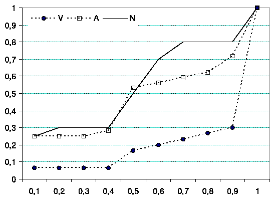
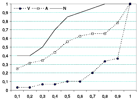
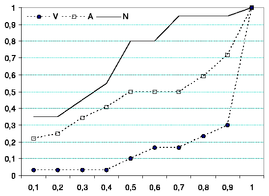
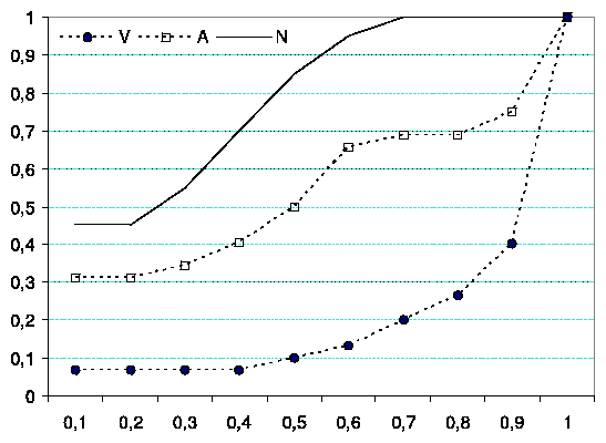
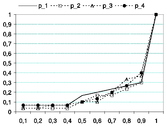
Figure 2: Cumulative Frequency of Choices per Lottery Panel; A: Addicts, V:
Victims, N: Normals.
Table 2: Between-subject analysis.
| Panel | | | |
| A. | 1 | 2 | 3 | 4 |
|
KRUSKAL-W c2 . | 15.48 | 27.62 | 30.74 | 29.87 |
| p-value | 0.00 | 0.00 | 0.00 | 0.00 |
| MEDIAN c2 | 16.82 | 25.31 | 34.00 | 35.20 |
| p-value | 0.00 | 0.00 | 0.00 | 0.00 |
| B. | | | | |
| Addicts vs. Victims | -3.34 | -3.58 | -3.82 | -3.61 |
| p-value | 0.00 | 0.00 | 0.00 | 0.00 |
| Victims vs. Normals | -3.52 | -5.15 | -5.36 | -5.29 |
| p-value | 0.00 | 0.00 | 0.00 | 0.00 |
| Addicts vs. Normals | -0.38 | -1.98 | -2.08 | -2.23 |
| p-value | 0.70 | 0.04 | 0.03 | 0.02 |
|
|
4 Results
a: Victims
b: Addicts
c: Normals
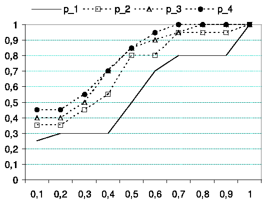
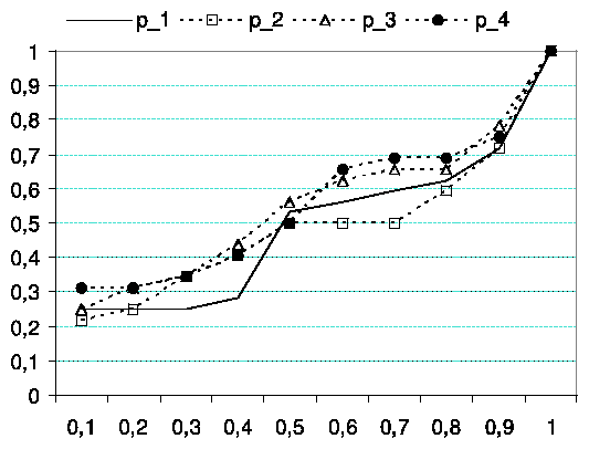
Figure 3: Choice differences across panels for Victims, Addicts & Normals (Cum. Freq.)
4.1 Differences in risk attitudes
First, we compare behavior across subject subsamples. Figures 2a-d present
cumulative frequencies of choices by subject subsample. Each figure presents
choices per lottery panel. The horizontal axis represents p, which is the
winning probability of a subject's preferred lottery. Notice that lotteries
are then ordered in the figures starting by the riskiest and finishing with
the certain outcome. The vertical axis represents the cumulative frequency
of choices. We can see how a very high percentage of victims (dashed line
with black dots) prefer the safe option (p=1) regardless of the panel.
We can see that the baseline population (normal subjects, continuous line)
is the riskiest (see, for example, the high percentage of people choosing p=0.1). Finally, in all panels, the behavior of addicts (dashed line with
square markers) lies between the behavior of the other two samples.
We can check, now, whether results are statistically different across
subsamples in each panel, based on a series of Kruskal-Wallis and Median
non-parametric tests for k=3 unrelated samples. The null hypothesis is
that the average (or the median) is the same in all the three subsamples
(victims, addicts and normals). We perform the same analysis in each panel.
Table 2 summarizes these tests.
Both series of tests yield identical results: samples are not drawn from the
same population. Neither the average nor the median can be considered
invariant across subject populations in any lottery panel. Each group's
behavior statistically differs from the other two subsamples' choices. A
series of Mann Whitney non-parametric tests for k=2 unpaired samples
report a similar message: with the exception of the comparison between
addicts and normals in panel 1 (where the risk-premium trade off is very
low) the remaining cases show differences among populations.6 Moreover in all the comparisons where victims are involved we see
that test are always significant differences for any value of a.
Table 2b shows this series of tests (the p-value is shown between
brackets):
Looking at each population's average choice across panels (victims =0.867,
addicts =0.560 and normals =0.385), we get that:
Result 1a: Addicts choose safer options than normal individuals, and:
Result 1b: The large majority of victims report themselves unwilling to take
any risk at all.
4.2 Behavior across panels
Now we explore within-subject behavior across lotteries. Figures, 3a-c show
cumulative distributions across panels for each subsample. Again, the
horizontal axis represents the winning probabilities of the lotteries chosen
(p), starting by the riskiest option and finishing with the sure outcome.
The vertical axis represents the cumulative frequency. Here we can observe
how behavior does not seem to significantly vary across panels for victims
(3-a) and addicts (3-b) while normals (3-c) seem to behave differently
across lottery panels.
Formal tests can be used to support these findings informing us on the
extent to which subjects within each subsample are sensitive to increases of
the risk-return parameter as we move from panel 1 to panel 4.
VICTIMS: Clearly, we do not observe any variation across panels; on
average their choices are 0.85 (panel 1, hereafter p1), 0.89 (p2), 0.87 (p3) and 0.86 (p4). Both the Friedman (c32=2.65;p=0.44 ) and Kendall (c32=2.65;p=0.44) tests for k=4 related samples do not reject the null hypothesis of equality of
distributions. Thus, we cannot reject the hypothesis that all samples are
drawn from the same population. Hence, victims do not react to the 4
different values of the risk-return parameter used to construct the four
panels.
ADDICTS: The invariant average behavior observed in the previous
group is also observed among addicts. The average behavior does not vary
across panels: 0.59 (p1), 0.59 (p2), 0.53 (p3) and 0.53 (p4). Both the Friedman (c32=2.62;p=0.45) and Kendall (c32=2.62;p=0.45) tests do not reject the null hypothesis. Hence,
addicts did not vary their behavior across panels.
NORMALS: In contrast to the other samples, our baseline
population reacted to the risk-return trade-off in the expected
way, choosing riskier lotteries as we move from panel 1 to panel
4. In the first panel (mean choice = 0.52) they behaved
similarly to addicts. However, they varied their choices when
they were faced with higher values of the risk-return parameter.
Therefore, in panels 2, 3 and 4 choice averages clearly fall:
0,38 (p2), 0,33 (p3) and 0,30 (p4). In contrast to
what we reported above on victims and addicts, both the Friedman
(c32=8.84;p=0.03) and Kendall (c32=8.84;p=0.03) tests reject the null hypothesis. Thus,
normal subjects do vary their behavior across panels.7
In a separate analysis, we defined premium sensitivity as the
slope of the best fitting line when choice was plotted against
panel (counting panels 1-4 as equally spaced). A higher slope
indicates a willingness to take more risk when the premium for
risk taking was higher. Premium sensitivity did not depend on
age, sex, or on overall risk attitude. It did, however, differ
significantly among the three groups by a simple analysis of
variance (F2,79=4.60, p=.013). Mean slopes (change in
response for each step from one panel to the next) were 0.000 for
victims, 0.023 for addicts, 0.070 for normals. Post-hoc
examination of the three pairs of groups showed a significant
difference only between victims and normals (F1,48=10.45,
p=.007, with Bonferroni correction). Addicts were in between,
with somewhat greater premium sensitivity (but not quite
significantly in this analysis) for those in the first year of
treatment than those in later years. (We discuss time in
treatment further, below.)
Table 3: Individual Behavior Model. Dependent Variable: pij (i's
choice in panel j)
| Variable | Coefficient | Std. Error | t-Statistic | Prob. |
|
C | 0.443966 | 0.034378 | 12.91430 | 0.0000 |
| PREMIUM | -0.004405 | 0.003738 | -1.178490 | 0.2395 |
| FIRST | 0.107583 | 0.050234 | 2.141624 | 0.0330 |
| MALE | -0.073739 | 0.013846 | -5.325516 | 0.0000 |
| GA | 0.149497 | 0.046938 | 3.184985 | 0.0016 |
| VICTIM | 0.470210 | 0.040997 | 11.46942 | 0.0000 |
|
R2=0.365123 | [`R]2=0.355265 | S.E. of Regression = 0.2835 | F-statistic = 37.03698 | Prob(F-statistic) = 0.00000 |
|
|
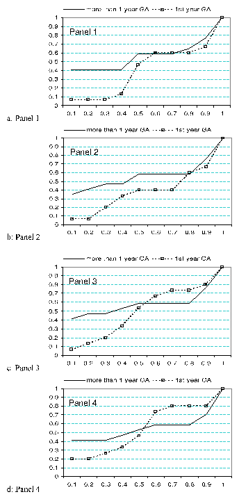 Figure 4: Panels 1-4. Comparison between PGs in the first year of treatment
and PGs under longer treatment periods (Cum. Freq.).
We summarize the preceding remarks as follows:
Result 2a: Both addicts and victims tend to maintain their
choices invariant across different scenarios of the risk-return
parameter.
Result 2b: Normal subjects' choices are sensitive to large risk-return
variations, and the normal subjects differ significantly from the
victims.
Figure 4: Panels 1-4. Comparison between PGs in the first year of treatment
and PGs under longer treatment periods (Cum. Freq.).
We summarize the preceding remarks as follows:
Result 2a: Both addicts and victims tend to maintain their
choices invariant across different scenarios of the risk-return
parameter.
Result 2b: Normal subjects' choices are sensitive to large risk-return
variations, and the normal subjects differ significantly from the
victims.
4.3 Effect of time in treatment
Figure 4 presents cumulative frequencies by panel of choices by PGs,
distinguishing between those who are in their first year of treatment and
those who have undergone treatment for longer periods. A more detailed
analysis of the time under treatment variable would be desirable, but
attempting this in our study would lead to excessively small subsamples for
each year. Therefore, both here and in the statistical model below we adopt
the dichotomous treatment of the variable.
However, it is also true that the first year of treatment is certainly
special and, as we will see, a significant effect of the first year
dummy is observed.8 Figure 5 presents the same data in a way
which allows us to observe the reaction of each type of PG to the different
values of the risk return parameter which were used to construct the four
panels. The risky decision making behavior of PGs in the first year of
treatment exhibits two major differences with respect to the behavior of PGs
under longer treatment periods: First, the former make safer options,
especially avoiding lotteries involving the riskiest bets. Second, while the
behavior of all other subjects remains largely invariant in the presence of
higher risk-return parameters, PGs in the first year of treatment are
strongly attracted by higher values of the risk-return parameter.
4.4 Overall analysis of individual differences
Finally, we study in a quantitative way the determinants of individual
decisions across the four panels. The estimation results reported in Table 3
refer to a model in which pij is subject i's choice in panel j � {1, 2, 3, 4}. The independent variables used are: a constant, C; the risk
premium rj used to construct panel j; a FIRST dummy taking the value
1 for gamblers under the first year of treatment and 0 otherwise; a MALE
dummy taking the value 1 for male subjects and 0 for female ones; GA is a
dummy taking the value 1 for gamblers under treatment and 0 otherwise; and
finally, a VICTIM dummy.
It is interesting to note that FIRST separates gamblers under the
first year of treatment from both normal subjects and gamblers
under longer treatment periods, as well as from victims. This is
inspired by the preceding discussion of figures 4 and 5,
according to which PGs under the first year of treatment are
those whose behavior differs most from that of normal subjects.
The regression results confirm that gamblers under the first year
of treatment make safer options than other subjects. Therefore,
PGs under longer periods of participation in GA sessions are not
so different from normal subjects.9
The remaining parameter estimates suggest that subjects who are indirectly
affected by gambling (victims) are willing to take fewer risks than all
other subjects. Also, as reported in most previous studies on gender
differences in risky choice, males are willing to take more risk than
females.
Finally, when all observations are pooled together, subjects exhibit limited
attraction (although on the expected direction) by higher returns to risk.
This finding contrasts with what was observed on Figure 5 above concerning
the behavior of PGs in the first year of treatment, exhibiting a strong
reaction to higher risk-return parameters. It also contrasts with our
finding reported in Result 2b concerning normal subjects' attraction by
large risk-return parameters.10
We summarize the results obtained from the aforementioned model estimation
together with some of the findings reported above on Figures 4 and 5 in the
following results.
Result 3a: Gamblers and victims exhibit significantly higher degrees of risk
aversion.
Result 3b: Gamblers in the first year of treatment are more risk averse than
those in posterior years of treatment, but they are attracted more than
other subjects by higher degrees of return to risk.
Result 3a is a synthesis of Results 1a and 1b, while Result 3b can be
interpreted as the consequence of some consciously egosyntonic behavior by
gamblers at an early stage of a psychological treatment. In fact, although
if there were more observations on each treatment year it would be
interesting to fit a nonlinear model, this finding indicates that the first
year of treatment is special, because probably subjects in early stages of
the treatment are more concerned with their self-image as people who are
free from their pathological attraction to risky bets. Their behavior in the
lottery choice task implemented in this study looks as if they were
committed to avoid taking risky bets, but they could not hide a secondary
element of their attraction to riskier bets when the returns to risk are
high.
Finally, we find that:
Result 4: Males are less risk-averse than females.
This result is compatible with numerous previous findings on the relation
between gender and risky decision-making.11
5 Conclusions
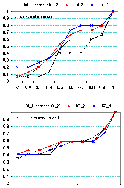 Figure 5: Comparison between PGs in the first year of treatment (top) and PGs under
longer treatment (bottom) with respect to their reactions to different risk-return
parameters.
This paper explores attitudes toward risk among two focus populations:
pathological gamblers under psychological treatment (
addicts") and gamblers' relatives (
victims"). We compare these subsamples to a control
population subsample ("normals"). Our
results can be summarized as follows:
Figure 5: Comparison between PGs in the first year of treatment (top) and PGs under
longer treatment (bottom) with respect to their reactions to different risk-return
parameters.
This paper explores attitudes toward risk among two focus populations:
pathological gamblers under psychological treatment (
addicts") and gamblers' relatives (
victims"). We compare these subsamples to a control
population subsample ("normals"). Our
results can be summarized as follows:
- Addicts are willing to take fewer risks than normal individuals.
- Victims are even more risk-averse than addicts and the majority of
them are unwilling to take any risk at all.
- Both addicts and victims maintain their choices invariant across
different scenarios of the risk-return trade-off.
- In contrast, normals' behavior presents the expected pattern of
choosing weakly riskier lotteries in the presence of a higher return to risk.
There is hardly any doubt that behavior in a risky task can be
explained as the result of a strategy aiming at what the subject
sees as the best option, after uncertainty and reward
attraction-repulsion have been accounted for. This issue has
been extensively studied so far under different theoretical
frameworks. However, our results indicate that the effects of a
given strategy or a decision making task as a whole on the
perception of oneself and others (Cross et al., 2002) also
matter. Gamblers who are voluntarily under treatment exhibit a
higher risk aversion than normal subjects, because probably they
feel that risky bets have already cost them a lot. In fact,
pathological gamblers in the first year of treatment appear to be
more risk averse than normal subjects, whereas as the number of
years under treatment increase, their degrees of risk taking
approach that of normal subjects. As we said before, this may be
the result of PGs' willingness to present themselves as totally
cured from their attraction to risky bets. However, our results
reveal a secondary element in a PG's behavior which should be
taken into account because it cannot be easily controlled by
consciously egosyntonic intentions. This element is attraction to
riskier bets in the presence of higher returns to risk. In that
aspect, PGs in the first year of treatment have exhibited the
strongest attraction to more profitable risky bets among all
other subjects studied here. Furthermore, the partners of PGs
under treatment, are even more unwilling to make risky bets, as
the majority of them take no risk at all.
Our results tend to confirm our main hypothesis. That is, our three
different subsamples behave differently in an abstract lottery-choice task.
The result concerning the victims is consistent with the psychological
literature focused on children's behavior living in a family where parental
gambling is a problem. However, it is not clear how addicts would behave if
real rewards were offered. We cannot give monetary prizes to gamblers under
treatment, but we can do it with people who go to casinos and are not under
medical supervision. This might be an interesting step for further research.
References
Albers, W., & Albers, G. (1983). On the prominence structure of
the decimal system. In Scholz, R. W. (Ed.), Decision
Making under Uncertainty, pp. 271-287. Elsevier North
Holland.
American Psychiatric Association. Diagnostic and
Statistical Manual of Mental Disorders. Third Ed. Washington
DC: American Psychiatric Press, 1980.
American Psychiatric Association. Diagnostic and
Statistical Manual of Mental Disorders. Fourth Ed. Washington
DC: American Psychiatric Press, 1994.
Battalio, R. C., Fisher, E., Kagel, J. H., Basmann, R. L.,
Winkler, R. C. & Krasner, R. (1973). A test of consumer demand
theory using observations of individual consumer purchases.
Western Economic Journal 11, 411-428.
Bosch-Domènech, A., Nagel, R. & Sánchez-Andrés, J.
V. (2005). Social Capabilities Preserved in Alzheimer Patients.
Working Paper, Universitat Pompeu Fabra.
Byrnes, J. P., Miller, D.C. & Schafer, W.D. (1999). Gender
differences in risk taking: A meta-analysis.
Psychological Bulletin, 125, 367-383.
Cartwright, C., Decaria, C., & Hollander, E. (1998).
Pathological gambling: A clinical review. Practical
Psychiatry and Behavioral Health 4, 277-286.
Cross, S. E., Morris. M. L. & Gore, J. S. (2002). Thinking about
oneself and others: The relational-interdependent self-construal
and social cognition. Journal of Personality and Social
Psychology 62, 399-418.
Darbyshire, P. (2001). The experience of pervasive loss: Children
and young people living in a family where parental gambling is a
problem. Journal of Gambling Studies 17, 23-45.
Eckel, C. and Grossman, P. (in press). Men, women and risk
aversion: Experimental evidence. In C. Plott and V. Smith
(Eds.), Handbook of Experimental Results. New York:
Elsevier.
Frost, R. O. (2001). Obsessive-compulsive features in
pathological lottery and scratch-ticket gamblers. Journal
of Gambling Studies 17, 5-19.
Gaboury, A. & Ladouceur, R. (1989). Erroneous perceptions and
gambling. Journal of Social Behavior and Personality,
4, 411-420.
García-Gallego, A., Georgantzís, N., Ginés, M. &
Jaramillo, A. (2006). Gender and risk attitudes in bargaining
experiments. Universitat Jaume I, mimeo.
Georgantzís, N., García-Gallego, A., Sabater-Grande, G.
& Genius, M. (2004). Lottery-specific risk attitudes:
Probability and reward attraction vs. risk-return tradeoffs.
Universitat Jaume I, mimeo.
Goodie, A. (2005). The role of perceived control and
overconfidence in pathological gambling. Journal of
Gambling Studies 21, 481-502.
Harris, C., Jenkins, M. & Glaser, D. (2006). Gender differences
in risk assessment: Why do women take fewer risks than men?
Judgement and Decision Making 1, 48-63.
Ladouceur, R., Arsenault, D., Freeston M.H. & Jacques, C.
(1997). Psychological characteristics of volunteers in studies
on gambling. Journal of Gambling Studies 13, 69-84.
Leopard, D. (1978). Risk preference in consecutive gambling.
Journal of Experimental Psychology: Human Perception and
Performance, 4, 521-528
Murningham, J. K., Roth, A. E., & Schoumaker, F. (1988). Risk
aversion in bargaining: An experimental study. Journal
of Risk and Uncertainty 1, 101-124.
Olsen, R. A. & Cox, C. M. (2001). The influence of gender on the
perception and response to investment risk: The case of
professional investors. The Journal of Psychology and
Financial Markets, 2, 29-36.
Pope, R. (1998). Attractions to and repulsions from chance. In
Leinfellner, W., Köhler E. (Eds.), Game Theory,
Experience, Rationality. Dordrecht: Kluwer, 95-107.
Pope, R. (2000). Evidence of deliberate violations of dominance
due to secondary satisfactions - Attractions to chance.
Homo Economicus, 14, 47-76.
Roth, A. & Malouf, M. W. K. (1979). Game-theoretic models and
the role of bargaining. Psychological Review 86,
574-594.
Sabater-Grande, G. & Georgantzis, N. (2002). Accounting for risk
aversion in repeated prisoners' dilemma games: An experimental
test. Journal of Economic Behavior and Organization,
48, 37-50.
Stinchfield, R.,Takushi, R., Hanson, G. & Bogan, S. (2003). A
program for the treatment of pathological gambling: Program
participation and treatment outcomes. Washington State
Department of Social and Health Services, RCW 67.70.350(5)
November 1.
Toneatto, T. (1999). Cognitive distortions in heavy gambling.
Journal of Gambling Studies, 13, 253-266.
Toneatto, T. (1999). Cognitive psychopathology of problem
gambling. Substance use and misuse, 34, 1593-1604.
Tversky, A. & Kahneman, D. (1982). Availability: A heuristic for
judging frequency and probability. In D. Kahneman, P. Slovic, &
A. Tversky (Eds.), Judgment Under Uncertainty: Heuristics
and Biases, pp. 163-178. Cambridge UK: Cambridge University
Press.
Appendix: Instructions
Welcome to this decision-making study. This session belongs to a research
project directed by Professors Nikolaos Georgantzís (Universitat Jaume
I) and Pablo Brañas (Universidad de Jaén and IESA-CSIC). Identical
sessions have been run in Valencia, Castellón, Crete and Athens. This
session is going to last 15 minutes. We thank you for your participation.
You are going to be asked to take four decisions. In the attached sheet
there are four panels [panels are in Figure 1]. Take for example the first
one. In the first row (P) you can see decimal numbers between 1 and 0.1
(both included). These numbers represent probabilities with which you can
hypothetically earn the amount of money shown in the cell below this number
(row "Xpuntos"). For instance, with probability 0.6 you can earn 1.73
EUR. Therefore, if you play this lottery:
- 60 out of 100 times you will earn 1.73 EUR
- 40 out of 100 times you will earn nothing.
However, if you look at the 0.3 cell you will see how payoffs are different:
- 30 out of 100 times you will earn 3.56 EUR
- 70 out of 100 times you will earn nothing.
You have to choose one of the 10 lotteries offered in this panel.
You have to do the same for each one of the other three panels.
When you are done, please fill the survey in sheet 3.
Thank you for your participation. As you can see you do not have to write
your name anywhere. This study is completely anonymous.
Footnotes:
1We are
grateful to Jon Baron for his support and advice, and two
anonymous referees. We would also like to thank Pilar
Sánchez-Olías, Jordi Brandts, Pedro Rey Biel, Al
Roth, and John Galvin. N. Georgantzís acknowledges
financial support by the Spanish Ministry of Education and
Science (SEJ2005-07544/ECON) and Bancaixa. Pablo
Brañas-Garza acknowledges financial support from DGICYT
(SEJ2004-07554/ECON).
Addresses: Pablo
Brañas-Garza, Dpto. de Teoría e Historia
Económica, Universidad de Granada, Spain
(pbg@ugr.es);
Nikolaos Georgantzís,
LINEEX/Laboratori d'Economia Experimental (LEE) and Dpto. de
Economia, Universitat Jaume I, Spain
(georgant@eco.uji.es);
Pablo Guillen,
Discipline of Economics, Faculty Economics and Business, The
University of Sydney (p.guillen@econ.usyd.edu.au)
2For example, Ladouceur et al. (2007) show that gamblers exhibit
an increased willingness to participate in studies on gambling.
3At the
moment of the experiment, they were heterogeneous with respect
to their times under psychological treatment: 15 of them were
in their "first year" under
treatment; 4 were in the second year; 2 in the third year; 5 of
them in the 5th; 2 in the 6th year; 2 in the 7th year and 2 had
been under treatment for over 10 years.
4We call gamblers'
spouses "victims" because
they are the ones who have suffered the negative consequences
of pathological gambling without having a gambling problem
themselves.
5However, there are many alternative
approaches which could explain our subjects' choices as
attraction to some prominent payof (Albers & Albers, 1983), a
subject's need to take some optimal degree of risk (Pope, 1998;
2000) or the result of some heuristic (Tversky & Kahneman,
1982) whose exhaustive review is beyond the scope of this
article.
6A series of Kolmogorov-Smirnov tests (non reported here) indicate identical
results.
7A
more detailed examination of this finding concerning normal
subjects can clarify the origin of the difference across
lottery panels. As we move from panel 1 to the following
panels, significant differences appear [Z-Wilcoxon tests for p1
vs. p2: -1.97 (p=0.04); p1 vs. p3: -2.24 (p=0.02); p1
vs. p4: -2.52 (p=0.01)]. However, the same test fails to
find any difference for the remaining comparisons [Z-Wilcoxon
tests for p2 vs. p3: -1.26 (p=0.20); p3 vs. p4: -0.59
(p=0.55); p2 vs. p4: -1.64 ( p=0.10 )]. That is, subjects are sensitive only to large
increases in the risk-return parameter.
8However a set of non-parametric Mann-Whitney test do not report clear
differences: panel 1 (Z=-1.26; p=0.23), panel 2 (Z=-1.23; p=0.23),
panel 3 (Z=-0.90; p=0.39), panel 4 (Z=-0.23; p=0.82). The largest
differences are observed in panels 1 and 2 however these differences
disappear for panels 3 and 4.
9For instance, in
panel 1, a Mann-Whitney test for differences between normal
subjects and PG's under more than one year of treatment yields
z=-0.26 with p-value=0.79.
10We have tried to deal with these effects in the framework of the model
reported in table 3. The introduction of a premium-subsample interaction
variable deals with these effects in a linear way which seems not to fit the
data sufficiently well.
11See for example, Byrnes et al. (1999), Harris et al. (2006)
for the case of financial risk, as well as the literature reviewed and
results reported by García-Gallego et al. (2005).
File translated from
TEX
by
TTH,
version 3.67.
On 21 Apr 2007, 05:05.